Chapter 3 Getting Started with Reactis
This chapter provides a quick overview of Reactis. It contains a brief description of each main component of the tool suite in the form of an extended “guided-tour” of the different features of the tool suite. Each “stop” in the tour is indicated by a §. The tour uses as a running example a simple Simulink / Stateflow model of an automobile cruise control that is included in the Reactis distribution.
3.1 A Note on Model Preparation
The cruise-control example included with the distribution does not require any special processing before you run Reactis on it; you may load the file immediately and start the guided tour. However, there is an important step that you should undertake when you are preparing models for use with Reactis. This section describes this preparatory step and discusses the Simulink operations needed to perform it.
Reactis supports a large portion of the discrete-time subset of Simulink and Stateflow. As it processes a Simulink / Stateflow model, it also interacts with MATLAB in order to evaluate MATLAB expressions, including references to workspace data items, that a model may contain.
In order for Reactis to process a model, Reactis must be able to automatically set up the MATLAB workspace data used by the model. For this reason, any workspace data items that a model uses must be initialized within one of the following locations (for more details see Section 14.1.1):
- Any Simulink model callback or block callback that is executed when loading or running the model (PreLoadFcn, PostLoadFcn, InitFcn, StartFcn).
- A “startup.m” file located in the folder where the model file is located.
- The Callbacks pane of the Reactis Info File Editor.
Below we describe how the workspace initialization was established in the cruise-control model file included in the Reactis release. In that example the MATLAB file cruise_constants.m defines two workspace variables that are used in the Simulink / Stateflow model file cruise.slx. The cruise_constants.m file was attached to cruise.slx using the following steps.
- Load cruise.slx into Simulink.
- In the Simulink window, select the File > Model Properties > Model Properties menu item1.
- In the resulting dialog, select the Callbacks tab.
- In the PreLoadFcn* section, enter cruise_constants; (note that the .m suffix is not included).
- Save the model.
This saved cruise.slx file is distributed with Reactis, so you do not need to undertake the above steps yourself in order to load and process this file in Reactis. The above steps are cited only for illustrative purposes.
3.2 Reactis Top Level
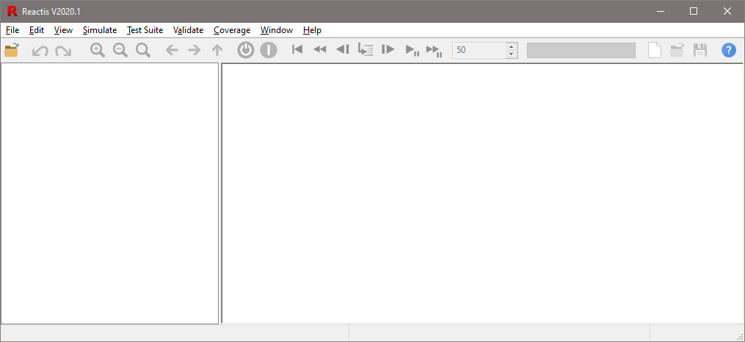
The Reactis top-level window contains menus and a tool bar for launching and
controlling verification and validation activities. Reactis is invoked as
follows.
| §1 | Select Start > All Programs > Reactis V2020.2 > Reactis from the Windows Start menu (or double-click on the desktop shortcut if you installed one). |
You now see a Reactis window like the one as shown in Figure
3.1. A model may be selected for analysis as
follows.
| §2 |
Click the
 (file open) button located at the leftmost
position on the tool bar. Then use the resulting file-selection
dialog to choose the file cruise.slx from the examples folder of
the Reactis distribution.2
(file open) button located at the leftmost
position on the tool bar. Then use the resulting file-selection
dialog to choose the file cruise.slx from the examples folder of
the Reactis distribution.2
|
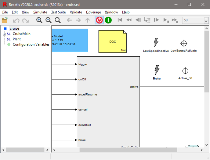
Loading the model causes the top-level window to change as shown in Figure 3.2. The panel to the right shows the top-level Simulink diagram of the model; the panel to the left shows the model hierarchy. In addition, the title bar now reports the model currently loaded, namely cruise.slx, and the Reactis info file (.rsi file) cruise.rsi that contains testing information maintained by Reactis for the model. Info files are explained in more detail in the next section (Section 3.3).
It is also worth noting that if during installation you chose to associate the .rsi file extension with Reactis, then you can start Reactis and open cruise.slx in a single step by double-clicking on cruise.rsi in Windows Explorer.
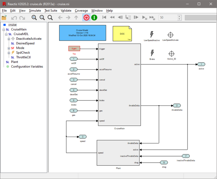
Subsystems in the hierarchy panel are tagged with icons indicating whether
they are Simulink (SL), Stateflow
(SF), Embedded MATLAB
(ML) 3, C source files
(C), C libraries
(LIB), S-Functions
(FN) 4,
assertions (
 ), or user-defined targets (
 ).
).
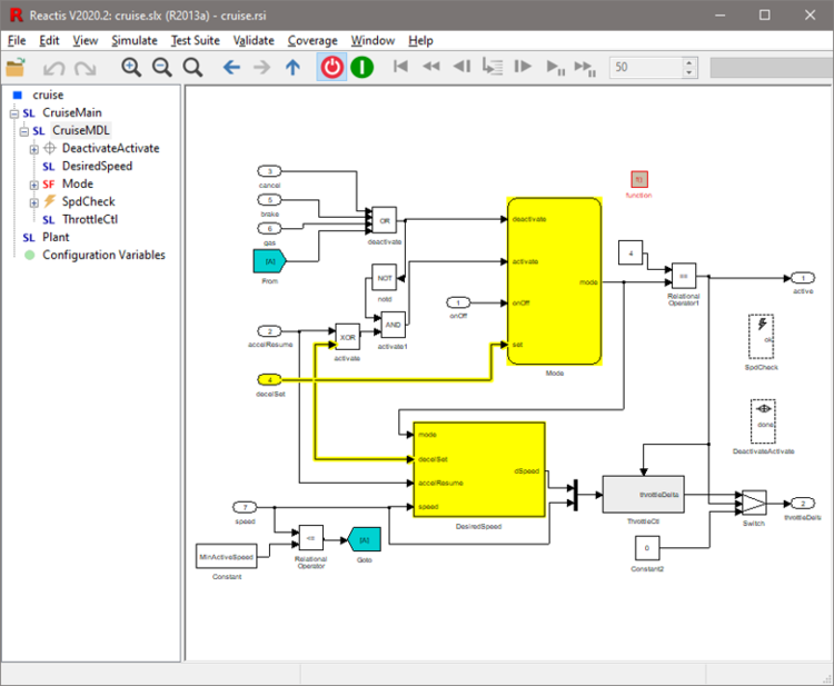
Reactis provides a signal-tracing mechanism which allows the path taken by a signal to be quickly identified. To trace a signal, left-click on any part of the signal line.
| §3 |
In the model hierarchy panel, left-click on the CruiseMDL subsystem, and
then, in the main panel, left-click on the on the signal line emerging
from the decelSet inport (inport 4). The result should be similar to
Figure 3.3. Click the
 button twice to
see how to trace the signal through different levels of the model hierarchy.
button twice to
see how to trace the signal through different levels of the model hierarchy.
|
As shown in Figure 3.3, signals are highlighted in yellow when left-clicked on. The route of the highlighted signal can then be easily identified. To turn off the highlighting, left-click on empty space in the main window.
3.3 The Info File Editor
Reactis does not modify the .slx file for a model. Instead the tool stores model-specific information that it requires in a .rsi file. The primary way for you to view and edit the data in these files is via the Reactis Info File Editor, which is described briefly in this section and in more detail in Chapter 5.
The next stop in the guided tour explains how this editor may be invoked on
cruise.rsi.
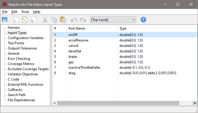
| §4 | Select the Edit > Inport Types... menu item. |
This starts the Reactis Info File Editor, as shown in Figure 3.4. Note that the contents of the .rsi file may only be modified when Simulator is disabled. When Simulator is running, the Info File Editor operates in read-only mode as indicated by “[read only]” in the editor window’s title bar.
.rsi files contain directives partitioned among the following panes in the Info File Editor.
- Harness.
- A harness specifies how a model is tested. The default
harness
[Top-Level]is for testing the full model. A harness can be created for any subsystem in a model by right-clicking on the subsystem and selecting Create New Harness.... - Inport Types.
- A type for each harness inport is used by Reactis to constrain the set of values fed into harness inports during simulation, test-case generation, and model validation. For example, you can specify an inport range by giving minimum and maximum values.
- Configuration Variables.
- Configuration variables are user-selected workspace data items which can change in between tests in a test suite (but not during a test).
- Test Points.
- Test points are internal signals which have been selected (by the user) to be logged in test suites.
- Outport Tolerances.
- Each outport of a harness may be assigned a tolerance. When executing a test suite on a model in Reactis Simulator, the tolerance specifies the maximum acceptable difference between the value computed by the model for the outport and the value stored in a test suite for the outport.
- General.
- Various settings that determine how a model executes in Reactis.
- Error Checking.
- Specify how Reactis should respond to various types of errors (e.g. overflow, NaN, etc.).
- Coverage Metrics.
- Specify which coverage metrics will be tracked for the model and adjust the configurable metrics (CSEPT, MC/DC, MCC, Boundary).
- Excluded Coverage Targets.
- Specify individual targets to be ignored when measuring the coverage of a model.
- Validator Objectives.
- Validator objectives (including assertions, user-defined targets, and virtual sources) are instrumentation that you may provide to check if a model meets its requirements. You can double-click on an item in this list to highlight the location of the objective in the model.
- C Code.
- If the Reactis for C Plugin is installed, this pane will contain information about C-coded S-functions, C code embedded within Stateflow charts and C library code called from either an S-function or Stateflow.
- External EML Functions.
- If the Reactis for EML Plugin is installed, this pane let’s you specify any external Embedded MATLAB functions used by your model (i.e. functions stored in .m files outside your model).
- Callbacks.
- These are fragments of MATLAB code that Reactis will run before or after loading a model in Simulink. Note, that these callbacks are distinct from those maintained by Simulink.
- Search Path.
- The model-specific search path is prepended to the global search path to specify the list of folders (for the current model) in which Reactis will search for files such as Simulink model libraries (.slx), MATLAB scripts (.m), and S-Functions (.dll, .mexw32, .m).
- File Dependencies.
- A list of files on which the current model depends. The file-dependency information enables Reactis to track changes in auxiliary model files so that information obtained from them for the purposes of processing the current model may be kept up to date. Typically, files listed here would include any .m files loaded as a result of executing the current model’s pre-load function. For example, a .m file mentioned in the pre-load function might itself load another .m file; this second .m file (along with the first) should be listed as a dependency in order to ensure that Reactis behaves properly should this .m file change. Dependencies on libraries (.slx files) are detected automatically and need not be listed here.
| §5 | To modify the type for an inport, select the appropriate row, then right-click on it and select Edit..., and make the desired change in the resulting dialog. Save the change and close the type editor by clicking Ok or close without saving by clicking Cancel. |
The types that may be specified are the base Simulink / Stateflow types extended with notations to define ranges, subsets and resolutions, and to constrain the allowable changes in value from one simulation step to the next. More precisely, acceptable types can have the following basic forms.
- Complete range of base type:
- By default the type
associated with an inport is the Simulink / Stateflow base type inferred from
the model. Allowed base types include:
int8,int16,int32,uint8,uint16,uint32,boolean,single,double,sfix*, andufix*. - Subrange of base type:
- bt[i, j], where bt is a Simulink / Stateflow base type, and i and j are elements of type bt, with i being a lower bound and j an upper bound.
- Subrange with resolution type:
- bt [i:j:k],
where bt is either
doubleorsingle, i is a lower bound, j is a resolution, and k is an upper bound; all of i, j and k must be of type bt. The allowed values that an inport of this type may have are of form i + n × j, where n is a non-negative integer such that i + n × j ≤ k. In other words, each value that an inport of this type may assume must fall between i and k, inclusive, and differ from i by some integer multiple of j. - Set of specific values:
- bt{ e1, … en }, where
bt is a base type and e1, … en are
either elements of type bt, or expressions of form v:w, where v is an
element of type bt and w, a positive integer, is a probability
weight. These weights may be used to influence the relative likelihood
that Reactis will select a particular value when it needs to select a
value randomly to assign to an inport having an subset type. If the
probability weight is omitted it is assumed to be “1”.
For example, an inport having type
uint{0:1, 1:3}would get the value 0 in 25% of random simulation steps and the value 1 in 75% of random simulation steps, on average. - Delta type:
- tp delta [i,j], where tp is either a base type, a range type, or a resolution type, and i and j are elements of the underlying base type of tp. Delta types allow bounds to be placed on the changes in value that variables may undergo from one simulation step to the next. The value i specifies a lower bound, and j specifies an upper bound, on the size of this change between any two simulation steps. More precisely, if a variable has this type, and v and v′ are values assumed by this variable in successive simulation steps, with v′ the later value, then the following mathematical relationship holds: i ≤ v′ − v ≤ j. Note that if i is negative then values are allowed to decrease as simulation progresses.
- Conditional type:
- if expr then tp1 else tp2, where expr is a Boolean expression and tp1 and tp2 are type constraints. If expr is true then the input assumes a value specified by tp1 otherwise it assumes a value specified by tp2. Currently, the only variable allowed in expr is the simulation time expressed as t.
Table 3.1 gives examples of types and the values they contain. For vector, matrix or bus inports, the above types can be specified for each element independently.
RSI Type Values in Type double [0.0,4.0]All double-precision floating-point numbers between 0.0 and 4.0, inclusive. int16 [-1,1]-1, 0, 1 int32 {0,4,7}0, 4, 7 uint8 {0:1,1:3}0, 1 double[0.0:0.5:2.0]0.0, 0.5, 1.0, 1.5, 2.0 int16 [0,3] delta [-1, 1]0, 1, 2, 3; inports of this type can increase or decrease by at most 1 in successive simulation steps. if t == 0 then double { 0.0 }else double [0.0,10.0]At simulation time zero, input has value 0.0; subsequently, input is between 0.0 and 10.0.
If any change is made to a port type, then “[modified]” appears in the title bars of the Info File Editor and the top-level Reactis window. You may save changes to disk by selecting File > Save from the Info File Editor or File > Save Info File from the top-level window.
If no .rsi file exists for a model, Reactis will create a default file the first time you open the Info File Editor, or start Simulator or Tester. The default type for each inport is the base type inferred for the port from the model. If you add or remove an inport to your model you can synchronize your .rsi file with the new version of the model by selecting Tools > Synchronize Inports, Outports, Test Points from the Info File Editor.
| §6 | Select the File > Exit menu item on the editor’s tool bar to close the Reactis Info File Editor. |
3.4 Simulator
Reactis Simulator provides an array of facilities for viewing the
execution of models. To continue with the guided tour:
| §7 |
Click the
 (enable Simulator) button in the tool bar
to start Reactis Simulator.
(enable Simulator) button in the tool bar
to start Reactis Simulator.
|
This causes a number of the tool-bar buttons that were previously disabled to become enabled.
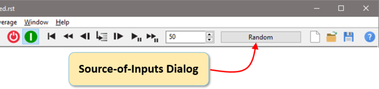
Simulator performs simulations in a step-by-step manner: at each simulation step inputs are generated for each harness inport, and resultant outputs reported on each outport. You can control how Simulator computes harness inport values using the Source-of-Inputs dialog as follows. Simulator may be directed to:
- generate values randomly (this is the default),
- query the user,
- read inputs from a Reactis test suite. Such tests may have been generated automatically by Reactis Tester, constructed manually in Reactis Simulator, or imported from a file storing test data in a comma-separated-value format.
To set the input source for an inport, use the Source-of-Inputs dialog located to the left of
 in the tool bar
(see Figure 3.5). The next part of the guided tour
illustrates the use of each of these input sources; interspersed with this
discussion are asides on coverage tracking, data-value tracking, and other
useful features.
in the tool bar
(see Figure 3.5). The next part of the guided tour
illustrates the use of each of these input sources; interspersed with this
discussion are asides on coverage tracking, data-value tracking, and other
useful features.
3.4.1 Generating Random Inputs
As the random input source is the default, no action needs to be taken
to set this input mode.
| §8 |
In the model hierarchy panel on the left of the Simulator window,
click on CruiseMain/CruiseMDL/Mode in order to display
the Stateflow diagram in the main window.
Then, click the
 (Run/Pause Simulation) button.
|
During simulation, blocks, signals, states, and transitions in the
diagram are highlighted in green as they are entered and executed.
The simulation stops automatically when the number of simulation steps
reaches the figure contained in the entry box to the left of the
Source-of-Inputs dialog. Before then, you may pause the simulation by clicking
the
(Run/Pause Simulation) button a second time.
Note, that simulation will likely pause in the middle of a simulation step.
You may then click:
-
 to continue executing a block at a time, or
-
 to complete the step, or
-
 to back up to the start of the step
The fast simulation button
 works like
, but
without animation, so simulation is much faster.
works like
, but
without animation, so simulation is much faster.
3.4.2 Tracking Model Coverage
While Simulator is running you may also track
coverage information regarding which parts of your model
have been executed and which have not.
These coverage-tracking features work for all input-source modes.
The next portion of the guided tour illustrates how these features are used.
| §9 | Make sure menu item Coverage > Show Details is selected (as indicated by a check mark in the menu). Select menu item Coverage > Show Summary. |
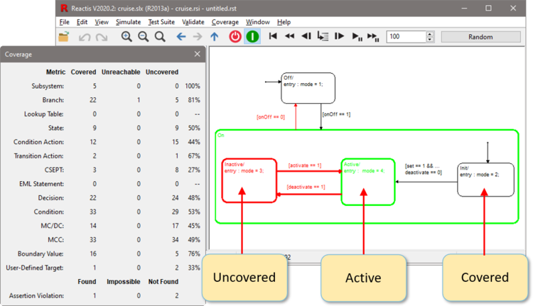
A dialog summarizing coverage of the different metrics tracked by
Reactis now appears. In the main panel, elements of the
diagram not yet exercised are drawn in red, as shown in Figure
3.6. Note that poor coverage is not uncommon with
random simulation. You may hover over a covered element to determine
the (1) test (in the case being considered here, the “test” is the
current simulation run and is rendered as . in the hovering
information) and (2) step within the test that first exercised the
item. This type of test and step coverage information is displayed
with a message of the form test/step.
You may view detailed information for the Condition, Decision and MC/DC
coverage metrics, which involve Simulink logic blocks and
Stateflow transition segments whose label includes an event and/or condition,
as follows.
| §10 |
Steps 1 and 2 below show how to open the Coverage Details dialog for
a decision on a Stateflow transition. Steps 3 through 6 demonstrate who to exclude
an individual coverage target from being tracked.
|
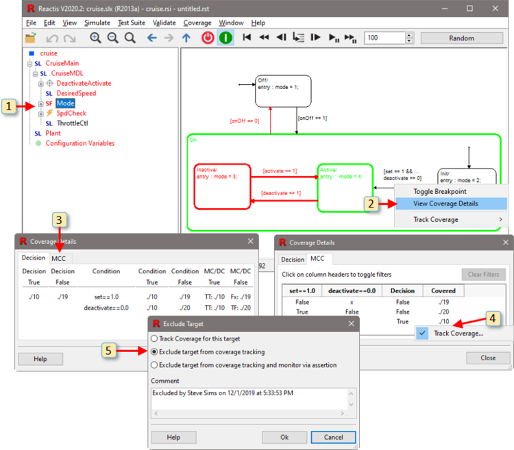
The Coverage Details dialog, shown in Figure 3.7, has two tabs: Decision and MCC. The Decision tab displays details for decision coverage, condition coverage, and MC/DC. The table in this figure gives information for the decision:
set == 1 && deactivate == 0
This decision contains two conditions:
-
set == 1 deactivate == 0
Conditions are the atomic boolean expressions that are used in decisions. The
first two columns of the table list the test/step information for when the
decision first evaluated to true and when it first evaluated to false. A value
-/- indicates that the target has not yet been covered.
The third column lists the conditions that make up the decision, while the forth
and fifth columns give test/step information for when each condition was
evaluated to true and to false.
MC/DC Coverage requires that each condition independently affect the
outcome of the decision in which it resides. When a condition has met the
MC/DC criterion in a set of tests, the sixth and seventh columns of the
table explain how. Each element of these two columns has the form b1 b2 ... bn:test/step, where bi reports the outcome of evaluating
condition i in the decision (as counted from left to right in the
decision or top to bottom in column three) during the test and step specified.
Each bi is either T to indicate the condition evaluated to true,
F to indicate the condition evaluated to false, or x to mean
the condition was not evaluated due to short circuiting.
The MCC tab of the Coverage Details dialog displays details of multiple condition coverage (MCC) which tracks whether all possible combinations of condition outcomes for a decision have been exercised. The table includes a column for each condition in the decision. The column header is the condition and each subsequent row contains an outcome for the condition: True, False, or x (indicating the condition was not evaluated due to short-circuiting). Each row also contains the outcome of the decision (True of False) and, when covered, the test and step during which the combination was first exercised.
It should be noted that the previous scenario relied on randomly generated input data, and replaying the steps outlined above will yield different coverage information than that depicted in Figure 3.7
An alternative way to query coverage information is to invoke the Coverage-Report Browser by selecting Coverage > Show Report. This is a tool for viewing or exporting coverage information that explains which model elements have been covered along with the test and step where they were first exercised. Yet another way to inspect test coverage is with Simulate > Fast Run With Report.... In addition to coverage data, these reports can contain other types of information such as plots showing expected outputs compared to actual outputs.
A simulation run, and associated coverage statistics, may be reset by
clicking the Reset to First Step button (
 ) in the tool
bar.
) in the tool
bar.
3.4.3 Reading Inputs from Tests
Simulation inputs may also be drawn from tests in a Reactis test
suite. Such a test suite may be generated automatically by Reactis
Tester, constructed manually in Reactis Simulator, or
imported from a file storing test-data in a comma-separated-value format. By
convention,
files storing Reactis test suites have a .rst filename extension.
A Reactis test suite may be loaded into Simulator as follows.
| §11 |
Click the
button in the tool bar to the right of the
Source-of-Inputs dialog and use the file-selection dialog to select
cruise.rst in the examples folder of the Reactis
distribution.
|
This causes cruise.rst, the name of a test suite file generated
by Reactis Tester, to appear in the title bar and the contents of the
Source-of-Inputs dialog to change; it now contains a
list of tests that have been loaded. To view this list:
| §12 |
Click on the Source-of-Inputs dialog (located to the left of
in the tool bar).
|
Each test in the suite has a row in the dialog that contains a test
number, a sequence number, a name, and the number of steps in the test.
Clicking the “all” button in the lower left corner specifies that
all tests in the suite should be executed one after another. To
execute the longest test in the suite:
| §13 |
Do the following.
|
If you look at the bottom-right corner of the window, you can see that the test
is being executed (or has completed), although the results of each execution
step are not displayed graphically. When the test execution completes, the
exercised parts of the model are drawn in black. If the Run
Simulation button (
) is clicked instead, then the results of each
simulation step are rendered graphically, with the consequence that simulation
proceeds more slowly.
Whenever tests are executed in Simulator, the value computed by the model for each harness outport and test point is compared against the corresponding value stored in the test suite. The tolerance for this comparison can be configured in the Info File Editor. An HTML report listing any differences (as well as any runtime errors encountered) can be generated by loading a test suite in Simulator and then selecting Simulate > Fast Run With Report.
3.4.4 Tracking Values of Data Items
When Simulator is paused5, you may
view the current value of a given data item (Simulink block
or signal line, Stateflow variable, Embedded MATLAB variable, or C variable) by hovering over
the item with your mouse cursor.
You may also select data items whose values you wish to track during
simulation using the watched-variable and scope facilities of
Simulator.
| §14 |
In the model hierarchy panel on the left of the Reactis window,
select the top-level of the model (“cruise”) for display. Then:
|
The bottom of the Simulator window now changes to that indicated in Figure 3.8.
The watched-variable panel shows the values of watched data items in the current simulation step, as does hovering over a data item with the mouse. Variables may be added to, and deleted from, the watched-variable panel by selecting them and right-clicking to obtain a menu. You may also toggle whether the watched-variable list is displayed or not by selecting the View > Show Watched Variables menu item.
Scopes display the values a given data item has assumed
since the beginning of the current simulation run. To open a scope:
| §15 |
Perform the following.
|
 button in the scope tool bar, so that the scope now appears similar
to Figure
button in the scope tool bar, so that the scope now appears similar
to Figure
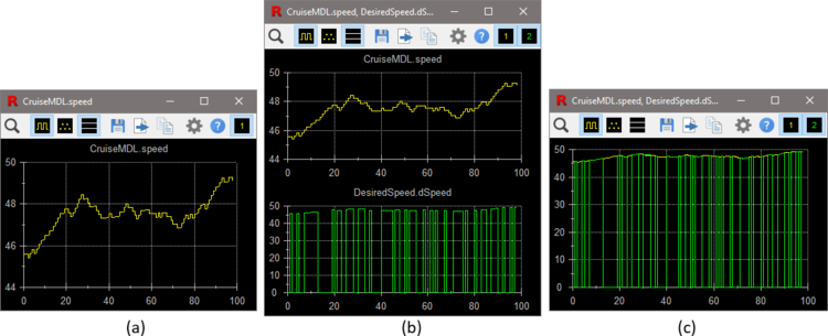
Scopes also have a zoom feature which is particularly useful for viewing the details of long signals. To zoom in, select a region of interest by clicking in the scope and dragging to specify a region. To scroll, hold down the control key, then click in the scope and drag. See Section 7.5.3 for more details on scopes.
| §16 |
Perform the following.
|
| §17 | Close the watched-variable panel by selecting the View > Show Watched Variables menu item. |
3.4.5 Querying the User for Inputs
The third way for Simulator to obtain values for inports
is for you to provide them. To enter this mode of
operation:
| §18 | Select User Guided Simulation from the Source-of-Inputs dialog. |
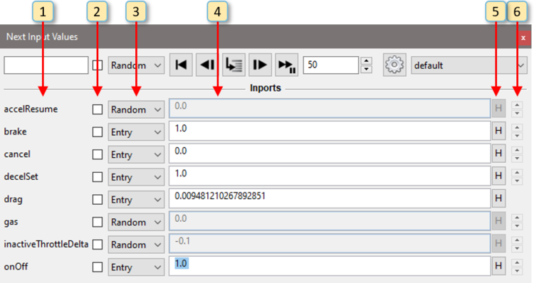
Upon selecting this input mode, a Next Input Values dialog
appears (as shown in Figure 3.10). This dialog lets you to specify
the input values for the next simulation step and see the values computed
for outputs and test points. Initially, each harness inport of the model
has a row in the dialog. You can remove inputs from the dialog or add
outputs, test points, and configuration variables by clicking the gear
button (
 ) in the toolbar of the Next Input Values dialog.
The row for each inport has six columns that determine the next input
value for the corresponding inport as follows.
) in the toolbar of the Next Input Values dialog.
The row for each inport has six columns that determine the next input
value for the corresponding inport as follows.
- The name of the item (inport, outport, test point, or configuration variable).
- This checkbox toggles whether the item is included in a scope displaying a subset of the signals from the Next Input Values dialog.
- This pull-down menu has several entries that determine
how the next value for the inport is specified:
- Random
- Randomly select the next value for the inport from the type given for the inport in the .rsi file.
- Entry
- Specify the next value with the text-entry box in column four of the panel.
- Min
- Use the minimum value allowed by the inport’s type constraint.
- Max
- Use the maximum value allowed by the inport’s type constraint.
- Test
- Read data from an existing test suite.
- If the pull-down menu in column three is set to “Entry”, then the next input value is taken from this text-entry box. The entry can be a concrete value (e.g. integer or floating point constant) or a simple expression that is evaluated to compute the next value. These expressions can reference the previous values of inputs or the simulation time. For example, a ramp can be specified by pre(drag) + 0.0001 or a sine wave can be generated by sin(t) * 0.001. For the full description of the expression notation see Section 7.4.1.
- If the pull-down menu in column three is set to “Entry”, then clicking the history button (labeled H) displays recent values the inport has assumed. Selecting a value from the list causes it to be placed in the text-entry box of column four.
- The arrow buttons in this column enable you to scroll through the possible values for the port. The arrows are not available for ports of type double or single or ranges with a base type of double or single.
When Run Fast Simulation
(
) is selected, the inport values specified
are used for each subsequent simulation step until the simulation is paused.
The toolbar at the top of the Next Input Values dialog includes
buttons for stepping (mini-step, single-step, fast simulation, reverse step, etc.)
that work the same as those in the top-level Simulator window. The text entry
box to the left of the toolbar lets you enter a search string to cause Reactis
to display only those items whose name contains the search string.
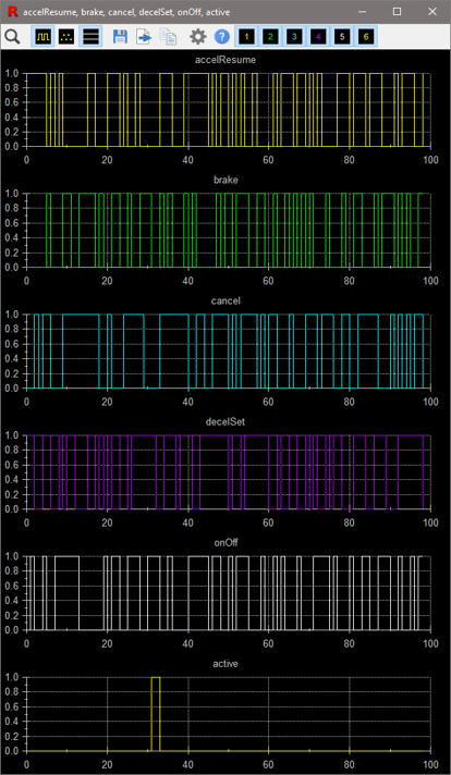
3.4.6 Constructing a Functional Test with User Guided Simulation
One use case for user guided simulation is for constructing functional tests. A test to ensure that the cruise control is enabled and disabled as expected can be created as follows.
| §19 |
In the following “Take a step” means click
in the
Next Input Values toolbar. Take n steps means click
n times.
|
3.4.7 Other Simulator Features
Simulator has several other noteworthy features. You may step both forward and backward through a simulation using toolbar buttons:
- The
button executes a single execution step.
- The
button executes the next “mini-step” (a
block or statement at a time).
- The
button, which causes the simulation to go back
(undo) a single step.
- The
 button causes the simulation to go back multiple
steps.
button causes the simulation to go back multiple
steps. - If using the Reactis for C Plugin with a model that includes C code, additional
buttons appear for stepping through C code:
 ,
,
 ,
,
 ,
,
 ,
,
 .
See Chapter 16, for a description of how these buttons work.
.
See Chapter 16, for a description of how these buttons work.
You may specify the number of steps taken when
,
, or
are pressed by adjusting the number in
the text-entry box to the right of
. When a simulation is paused at the end of a
simulation step (as opposed to in the middle of a simulation step),
the current simulation run may be added to the current test suite by
selecting the menu item Test Suite > Add/Extend Test. After
the test is added it appears in the Source-of-Inputs dialog. After saving the
test suite with Test Suite > Save, the steps in the new test
may be viewed by selecting Test Suite > Browse. A model (or
portion thereof, including coverage information) may be printed by
selecting File > Print....
Breakpoints may be set by either:
- right clicking on a subsystem or state in the hierarchy panel and selecting Toggle Breakpoint; or
- right clicking on a Simulink block, Stateflow state, or Stateflow transition in the main panel and selecting Toggle Breakpoint. Additionally, if you are using the Reactis for EML Plugin or the Reactis for C Plugin, then a breakpoint may be set on any line of C/EML code that contains a statement by right-clicking just to the right of the line number and selecting Toggle Breakpoint.
The
 symbol is drawn on a model item when a break point is set.
During a simulation run, whenever a breakpoint is hit, Simulator pauses
immediately.
symbol is drawn on a model item when a break point is set.
During a simulation run, whenever a breakpoint is hit, Simulator pauses
immediately.
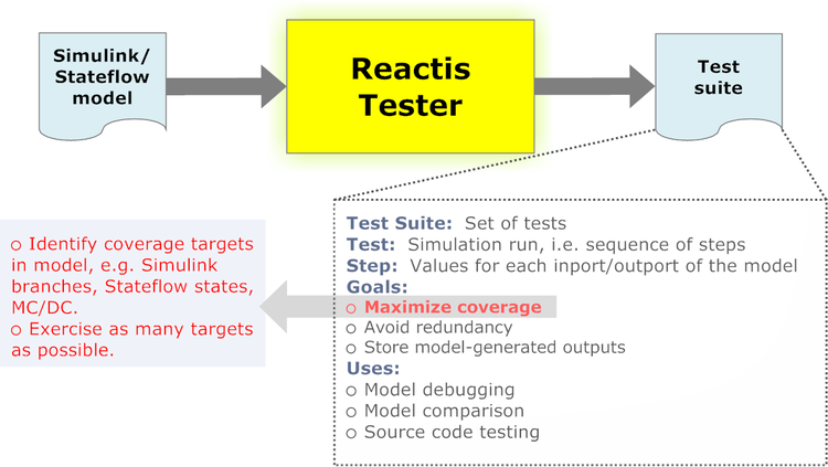
3.5 Tester
Tester may be used to generate a test suite (a set of tests) automatically from a Simulink / Stateflow model as shown in Figure 3.12. The tool identifies coverage targets in the model and aims to maximize the number of targets exercised by the generated tests.
To start Tester:
| §20 | Select the Test Suite > Create menu item. |
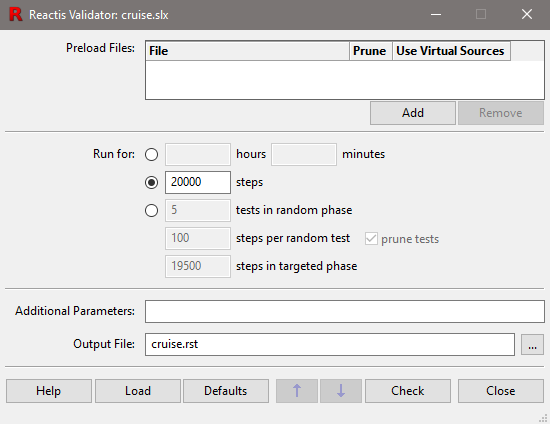
This causes the window shown in Figure 3.13 to appear. If you specify existing test suites in the Preload Files section, Tester will execute those suites, then add additional test steps that exercise targets not covered by the preloaded suite(s). The second section (Run for) determines how long Tester should run. The third section (Coverage Objectives) lists the metrics which Tester will focus on. In the fourth section, you specify the name of the output file in which Tester will store the new test suite (Output File).
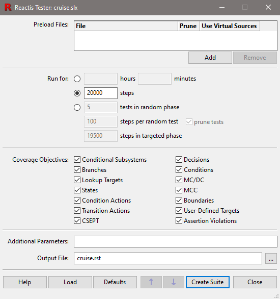
There are three options provided in the Run for section. The default option, as shown in Figure 3.13, is to run Tester for 20,000 steps. Alternatively, you may choose to run Tester for a fixed length of time by clicking on the top radio button in the Run for section, after which the steps entry box will be disabled and the hours and minutes entry boxes will be enabled. These values are added together to determine the total length of time for which Tester will run, so that entering a value of 1 for hours and 30 for minutes will cause Tester to run for 90 minutes. See Chapter 8 for usage details of the less-often used third radio button in the Run for section.
The Coverage Objectives section contains check boxes which are used to select the kinds of targets Tester will focus on while generating tests. Chapter 6 describes the different types of coverage tracked by Reactis.
To generate a test suite in the guided tour, retain the default
settings and:
| §21 | Click the Create Suite button. |
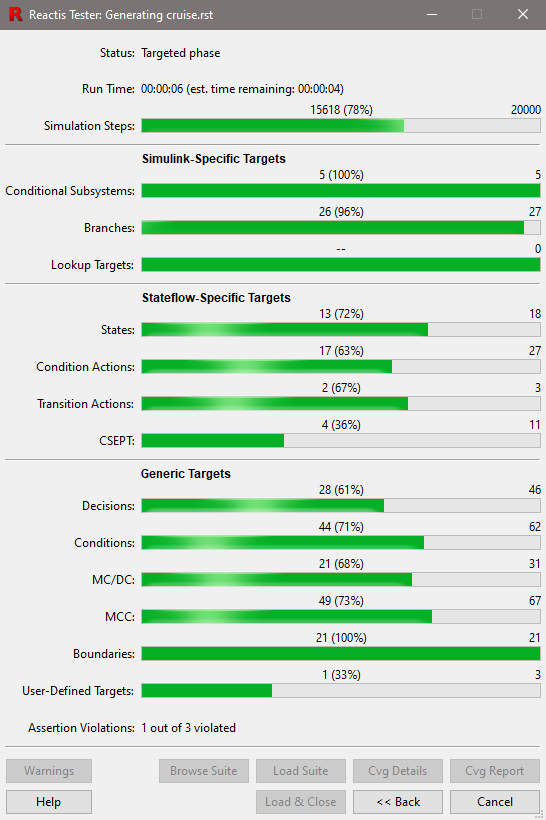
The Tester progress dialog, shown in Figure 3.14, is displayed during test-suite generation. When Tester terminates, a results dialog is shown, and a file cruise.rst containing the suite is produced. The results dialog includes buttons for loading the new test suite into the Test-Suite Browser (see below) or Reactis Simulator.
3.6 The Test-Suite Browser
The Test-Suite Browser is used to view the test suites created by Reactis. It may be invoked from either the Tester results dialog or the Reactis top-level window.
| §22 | Select the Test Suite > Browse menu item and then cruise.rst from the file selection dialog that pops up. |
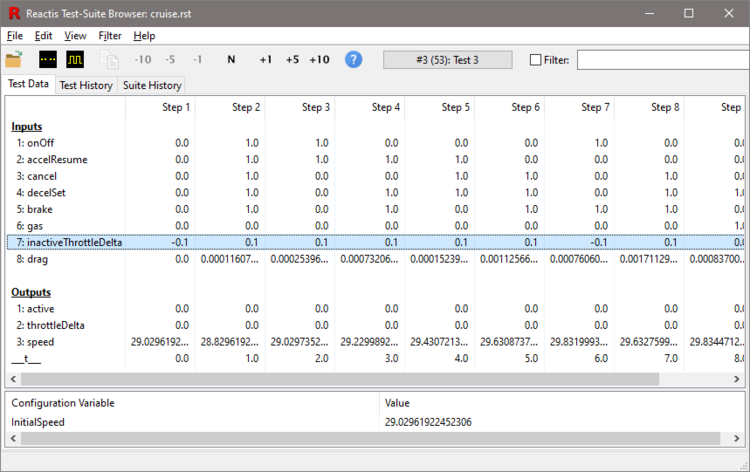
A Test-Suite Browser window like the one shown in Figure 3.15 is
then displayed. The Test Data tab of the browser displays
the test selected in the button/dialog located near the center of the
browser’s tool bar. The main panel in the browser window shows the
indicated test as a matrix, in which the first column gives the names of
input and output ports of the model and each subsequent column lists the
values for each port for the corresponding simulation step. The simulation
time is displayed in the output row labeled “___t___”. The
buttons on the tool bar may be used to scroll forward and backward in the
test. The Test History and Suite History tabs display
history information recorded by Reactis for the test and the suite as a
whole.
The Filter entry box on the right side of the toolbar lets you search
for test steps that satisfy a given condition. You enter a boolean expression
in the search box and then select the filter check box to search for test steps
in the suite for which the expression evaluates to true. For example, to see
each step where the cruise control is active enter “active == 1” and
then select the Filter check box.
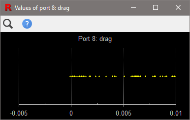
The Test-Suite Browser may also be used to display the entire set of values
passing over a port during a single test or set of tests.
| §23 |
Perform the following in the Test-Suite Browser window.
|
A dialog similar to that shown in Figure 3.16 appears. In the figure, each value assumed by the inport drag is represented by a yellow dot.
3.7 Validator
Reactis Validator is used for checking whether models behave correctly. It enables the early detection of design errors and inconsistencies and reduces the effort required for design reviews. The tool gives you three major capabilities.
- Assertion checking.
- You can instrument your models with assertions, which monitor model behavior for erroneous scenarios. The instrumentation is maintained by Reactis; you need not alter your .slx file. If Validator detects an assertion violation, it returns a test highlighting the problem. This test may be executed in Reactis Simulator to uncover the source of the error.
- Test scenario specifications.
- You can also instrument your models with user-defined targets, which may be used to define test scenarios to be considered in the analysis performed by Tester and Validator. Like assertions, user-defined targets also monitor model behavior; however, their purpose is to determine when a desired test case has been constructed (and to guide Reactis to construct it), so that the test may be included in a test suite.
- Concrete test scenarios.
- Finally, you can place virtual sources at the top level of a model to control one or more top-level inports as a model executes in Reactis. That is, you can specify a sequence of values to be consumed by an inport during simulation or test-generation. Virtual sources can be easily enabled and disabled. When enabled, the virtual source controls a set of inports and while disabled those inports are treated by Reactis just as normal top-level inports.
Conceptually, assertions may be seen as checking system behavior for potential errors, user-defined targets monitor system behavior in order to check for the presence of certain desirable executions (tests), and virtual sources generate sequences of values to be fed into model inports. Syntactically, Validator assertions, user-defined targets, and virtual sources have the same form and are collectively referred to as Validator objectives.
Validator objectives play key roles in checking a model against requirements given for its behavior. A typical requirements specification consists of a list of mandatory properties. For example, a requirements document for an automotive cruise control might stipulate that, among other things, whenever the brake pedal is depressed, the cruise control should disengage. Checking whether or not such a requirement holds of a model would require a method for monitoring system behavior to check this property, together with a collection of tests that would, among other things, engage the cruise control and then apply the brake. In Validator, the behavior monitor would be implemented as an assertion, while the test scenario involving engaging the cruise control and then stepping on the brake would be captured as a user-defined target.
3.7.1 Manipulating Validator Objectives
This section gives more information about Validator objectives.
| §24 |
Do the following.
|
 button in the
top-level toolbar. (Validator objectives may only be modified or
inserted when Simulator is disabled.)
button in the
top-level toolbar. (Validator objectives may only be modified or
inserted when Simulator is disabled.)
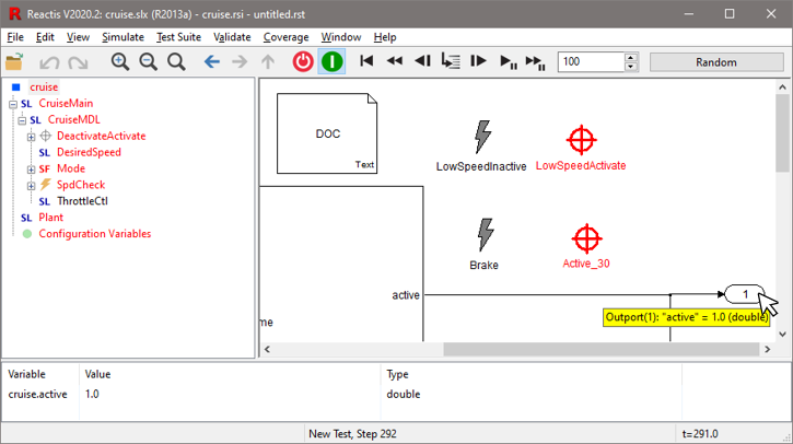
After performing these operations, you now see a window like the one
depicted in Figure 3.17. The three kinds of objectives are
represented by different icons; assertions are denoted by a lightning bolt
, targets are marked by a cross-hair symbol
, and virtual sources are represented by
 .
.
Validator objectives may take one of two forms.
- Expressions.
- Validator supports a simple expression language for defining assertions, user-defined targets, and virtual sources.
- Simulink / Stateflow observer diagrams.
- Simulink / Stateflow diagrams may also be used to define objectives. Such a Simulink subsystem defines a set of objectives, one for each outport of the subsystem. For assertion diagrams, a violation is flagged by a value of zero on an outport. For user-defined targets, coverage is indicated by the presence of a non-zero value on an outport. For virtual sources, each outport controls an inport of the model.
To see an example expression objective, do the following.
| §25 | Right click on the Brake assertion and select Edit Properties. When through with this step, click Cancel to dismiss the dialog. |
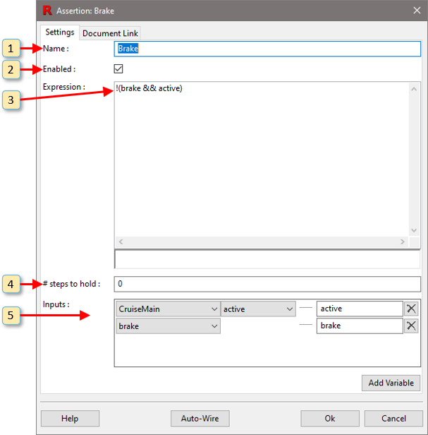
A dialog like that shown in Figure 3.18 now appears. This dialog shows an expression intended to capture the following requirement for a the cruise control: “Activating the brake shall immediately cause the cruise control to become inactive.” Note that the dialog consists of five parts:
- Name. This name labels the assertion in the model diagram.
- Enabled. This check box enables and disables the expression.
- Expression. This is a C-like boolean expression. The interpretation of such an assertion is that it should always remain “true”. If it becomes false, then an error has occurred and should be flagged. In this case, the expression evaluates to “true” provided that at least one of brake and active is false (i.e. the conjunction of the two is false). Section 9.3.1 contains more detail on the expression notation.
- # steps to hold. For assertions, this entry is an integer value that specifies the number of simulation steps that the expression must remain false before flagging an error. For user-defined targets, the entry specifies the number of steps that the expression must remain true before the target is considered covered.
- Inputs. The entry boxes in the right column of this section list
the variables used to construct the expression. These can
be viewed as virtual input ports to the expression objective. The
pull-down menus to the left of the section specify which data items
from the model feed into the virtual inputs. Note that, although you
can manually specify the inputs and wiring within this dialog, it is
simpler to:
- Leave this section blank when creating an objective.
- After clicking Ok to dismiss the dialog, drag and drop signals from the main Reactis panel onto the objective.
To see an example diagram objective:
| §26 |
Perform the following.
|
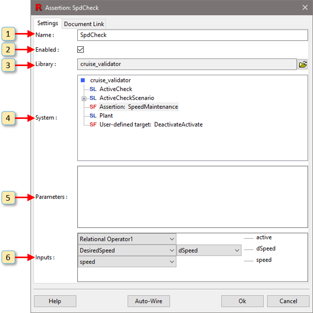
A dialog like the one in Figure 3.19 now appears. This dialog contains five sections.
- Name. The name of the objective.
- Enabled. This check box enables and disables the objective.
- Library. The Simulink library containing the diagram for the objective. In the case of SpdCheck, the target resides in cruise_validator.slx.
- System. The system in the library that is to be used as the objective. In this case, the system to be used is SpeedMaintenance.
- Parameters. If the subsystem selected for use as an objective is a masked subsystem, then this panel is used to enter the relevant parameters. In the case of SpdCheck, no parameters are required because the indicated subsystem is not masked.
- Inputs. The wiring panel is used to indicate which data items in
the model should be connected to the inputs of the objective. In this case,
SpdCheck has three inputs: speed, dSpeed, and
active. The wiring information indicates that the first input should be
connected to (the output of) Relational Operator1; the second should be
connected to the dSpeed output of subsystem DesiredSpeed; and
the third input should be connected to the speed inport of the current
level of the model. In general, this panel contains pull-downs describing all
valid data items in the current scope to which inputs of the objective may be
connected.
Note, that, although you can manually specify the wiring within this dialog, it is simpler to:
- Leave the wiring unspecified after inserting an objective.
- After clicking Ok to dismiss the dialog, drag and drop signals from the main Reactis panel onto the objective.
Wiring information may be viewed by hovering over a diagram objective in the main Reactis model-viewer panel.
Diagram-based objectives may be viewed as monitors that read values from the model being observed and raise flags by setting their outport values appropriately (zero for false, non-zero for true). A diagram-based assertion in essence defines one “check” for each of its outports, with such an outport check being violated if it ever assumes the value zero. Similarly, a diagram-based target objective in essence defines one “target” for each outport; such a target is deemed covered if it becomes non-zero.
To view the diagram associated with SpdCheck:
| §27 |
Perform the following.
|
These operations display the Stateflow diagram shown in Figure 3.20. This diagram encodes the following requirement: “While it is engaged, the cruise control shall not allow the desired and actual speeds to differ by more than 1 mile per hour for more than three time units.”
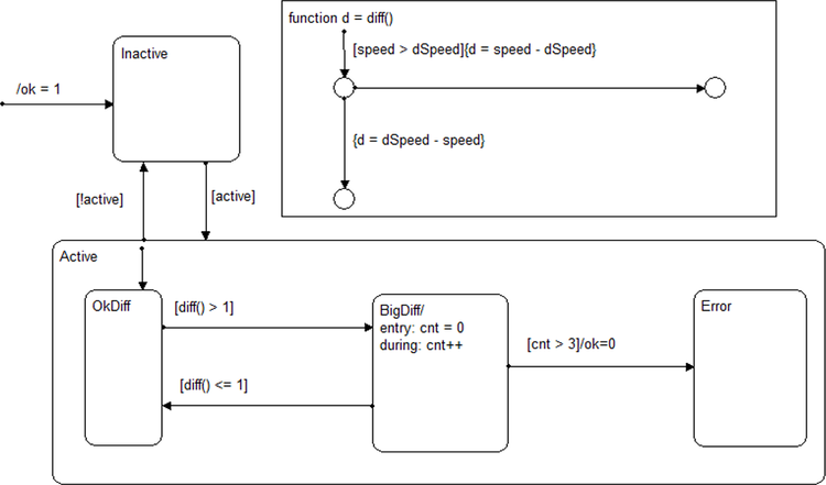
To understand how this diagram captures this requirement, note that the SpdCheck diagram has two top-level states, one corresponding to when the cruise control is active and one when it is inactive. The active state has three child states:
- OkDiff
- Control resides here when the difference between actual and desired speed is within the accepted tolerance.
- BigDiff
- Control resides here when the difference between actual and desired speed is greater than the accepted tolerance, but three time units have not yet elapsed.
- Error
- Control resides here when the difference between actual and desired speed has been greater than the accepted tolerance for more than three consecutive time units.
Note that the transition action executed as state Error is entered sets the outport ok to 0. This is how an assertion violation is flagged.
Diagram objectives give you the full power of Simulink / Stateflow to formulate assertions and targets. The objectives may use any Simulink blocks supported by Reactis, including full Stateflow. The diagrams are created using Simulink and Stateflow in the same way standard models are built; they are stored in a separate .slx file from the model under validation.
Diagram wiring is managed by Reactis, so the model under validation need not be modified at all. As this information is stored in the .rsi file associated with the model, it also persists from one Reactis session to the next. After adding a diagram objective to a model, the diagram is included in the model’s hierarchy tree, just as library links are. See Chapter 9 for more details on using Reactis Validator.
3.7.2 Launching Validator
To use Validator to check for assertion violations:
| §28 | Select the Validate > Check Assertions... menu entry. |
A dialog like the one in Figure 3.21 now appears. The dialog is similar to the Tester launch screen in Figure 3.13 because the algorithms underlying the two tools are very similar. Conceptually, Validator works by generating thorough test suites from the instrumented model using the Tester test-generation algorithm and then applying these tests to the instrumented model to see if any violations occur. Note that when a model is instrumented with Validator objectives, the test-generation algorithm uses the objectives to direct the test construction process. In other words, Reactis actively attempts to find tests that violate assertions and cover user-defined targets. Validator stores the test suite it creates in the file specified in this dialog. The tests may then be used to diagnose any assertion violations that arise.
Note that if a model is instrumented with Validator objectives Reactis Tester also aims to violate the assertions and cover the user-defined targets.
- 1
- Prior to R2012b, the dialog was invoked via menu item File > Model Properties...
- 2
- Reactis supports the older .mdl model file format in the same way support is described here for .slx files.
- 3
- Embedded MATLAB only shows up if you are using the Reactis for EML Plugin
- 4
- C code subsystems only show up if you are using the Reactis for C Plugin
- 5
- A simulation is paused if Simulator is not actively computing simulation step(s).