8. Reactis Simulator#
Simulator provides an array of features — including single- and multi-step forward and backward execution, breakpoints, simulations driven by Tester-generated test suites, and interactive simulation — for simulating your source code. The tool also allows visual tracking of coverage data and the values data items assume during simulation.
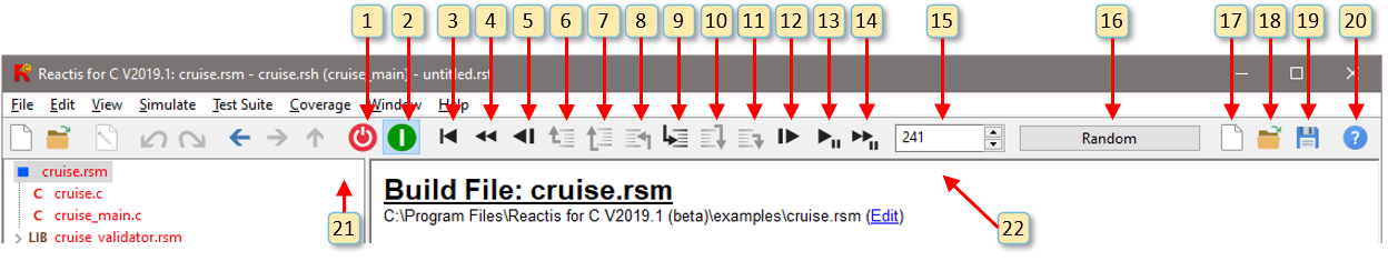
Fig. 8.1 The Reactis Simulator toolbar.#
Figure 8.1 contains an annotated screen shot of the Simulator toolbar. Some of the buttons and menus on the leftmost part of the window have been elided; The Reactis for C Top-Level Window chapter contains descriptions of these items. The next section describes the labeled items in Figure 8.1, while the section following discusses the menu entries related to Simulator. The subsequent sections discuss the different modes for generating inputs during simulation, the ways to track data values, how to monitor code coverage, the importing and exporting of test suites, and the different code highlighting styles used by Simulator.
8.1. Labeled Window Items#
Disable Reactis Simulator.
Enable Reactis Simulator.
Clicking this button resets the simulation; the code execution is returned to the start state, and coverage information is appropriately reset.
Clicking this button causes the simulation to take n steps back, where n is specified by window item 15. Coverage information is updated appropriately upon completion of the last backward step.
Clicking this button causes the simulation to take one step back. Coverage information is updated appropriately.
Step backward to the point just before the current function was called.
Step backward one statement. Any function calls performed by the statement are stepped over.
Step backward one statement. If the statement performed any function calls, stop at the end of the last function which was called.
Clicking this button executes a single C statement, stepping into a function when at a function call. The button is disabled during fast simulation and reverse simulation.
When paused at a function call, clicking this button steps over the function (executes the function and pauses at the following statement).
Step out of the currently executing function.
Clicking this button causes the simulation step to advance forward by one full step; that is, values are read on the harness inputs, the program’s response is computed and values are written to the harness outputs. If a step has been partially computed, then execution picks up with the current partially computed step and continues until the end of the step, at which point values are written to the harness outputs.
When paused, clicking this button causes n forward simulation steps to be taken, where n is specified by window item 15. The diagram in the main panel is updated during simulation to reflect the currently executing code. When Coverage > Show Details is selected, coverage targets will change from red to black as they are covered during the simulation run. If the end of the current test or test suite is reached or you click the Run/Pause button again (window item 13), then simulation stops at the end of the current simulation step.
Clicking this button causes n simulation steps to be executed, where n is specified by window item 15. The diagram in the main panel is not updated while the simulation is in progress but is updated when simulation halts. If the end of the current test or test suite is reached then simulation halts.
When a fast simulation is running, clicking this button pauses the simulation and the end of the currently executing step.
This window item determines how many steps are taken when buttons corresponding to window items 4, 13, or 14 are clicked. When the Source-of-Inputs Dialog (window item 16) is set to a test or test suite, the number of steps may be set to 0 to indicate that the entire test or test suite should be executed.
The Source-of-Inputs Dialog determines how input values are computed during simulation. See the Specifying the Simulation Input Mode section for details.
Clicking this button causes a new, empty test suite to be created. The name of the
.rstfile containing the suite is initially“unnamed.rst”and is displayed in the title bar of the Reactis for C window.
Clicking this button displays a dialog for selecting a test-suite (
.rstfile) to be loaded into Simulator. After it is loaded, the test suite’s name is displayed in the title bar, and the tests are listed in the Source-of-Inputs Dialog (window item 16).
Clicking this button causes the current test suite to be saved.
View Reactis for C help.
The hierarchy panel (partially shown) supports the navigation of the project, as described in the Labeled Window Items section. It shows the root build file (
.rsmfile) at the top, and the C files and libraries below.
The main panel (partially shown) displays the contents of the C or
.rsmfile currently selected in the hierarchy panel. You may interact with the panel in a number of different ways using the mouse. These include hovering over items in the code (e.g. variables, function names, macros) or right-clicking in various parts of the panel. The following mouse operations are available when Simulator is enabled:
- Hovering…
over a variable name (global or local) or function parameter displays [1]1:
the current value of the variable or “[out of scope]” if the variable is not currently in scope.
where the variable is defined.
where the variable was last modified.
over a function name displays the return type and types of its parameters along with the location of the function definition.
over a macro name in a macro invocation displays the expansion of the macro.
over a typedef shows the typedef declaration.
over the argument of a
#includedirective displays the pathname of the file which was included.over any Reactis coverage target will display the test and step within the test during which the target was first executed. This information is presented in a message of the form “Covered: test/step”. A “.” in the test location indicates the current simulation run. For boundary value coverage, you may hover over the definition of inputs or configuration variables. In the case of inputs, this is either the definition of a parameter of the entry function or a global variable declaration. In the case of configuration variables, this is a global variable declaration.
For more details on querying coverage information see the Tracking Code Coverage section, The Reactis Coverage-Report Browser chapter, and the Reactis Coverage Metrics chapter.
- Right Clicking…
Causes different pop-up menus to be displayed. The contents of the menus vary based on where the click occurs and whether or not Simulator is enabled. A summary of the menu items available when Simulator is enabled follows [2]. For descriptions of the menu entries available when Simulator is disabled, see the Labeled Window Items section.
Right-Click Location |
Menu Entries (when Simulator is enabled) |
|---|---|
Global variable or static local variable |
|
Decision coverage target |
|
Harness output |
|
In the line number bar to the left of the main panel. |
|
- Double Clicking…
in the line number bar to the left of the main panel toggles a breakpoint for the line.
on any other item opens a separate window which contains the same information displayed when hovering on that item. This is useful when the information in in the hover window is clipped due to excessive length.
8.2. Menus#
Except for the documented exceptions related to editing .rsh files
[3], the menus described in the Menus section work in the same
manner when Simulator is enabled. The following additional menu items
are also active when Simulator is enabled.
- View menu.
The following entries become enabled when Simulator is “on”.
- Show Watched Variables.
Toggle whether or not watched-variable list is displayed. The default is not to show them; adding to the list automatically causes the list to be displayed.
- Clear Watched Variables.
Remove all items from the watch list.
- Open Difference Scopes…
Open a difference scope on one or more harness outputs. This item is only enabled when the input source is a test suite. See the Difference Scopes sections for details.
- Close All Scopes.
Close all open scopes.
- Open Scope (Signal Group)
Open a scope on a signal group. A signal group is created by clicking the save button
 in a scope to save the
current configuration of the scope as a signal group (set of signals
along with the scope settings for displaying them).
in a scope to save the
current configuration of the scope as a signal group (set of signals
along with the scope settings for displaying them).- Delete Signal Group
Delete a signal group.
- Save Profile as…
Save the current view profile under a new name. The view profile contains the currently opened scopes and watched variables. Profiles are saved in with the
.rspsuffix.
- Load Profile…
Load a different view profile (
.rspfile ). This will automatically open all scopes and watched variables stored in the profile.
- Simulate menu.
The following entries are available when Simulator is enabled.
- Simulator on/off.
Enable or disable Simulator. When disabled, Simulator behaves as a source code viewer; that is, the code can be viewed but simulation capabilities are disabled.
- Fast Run with Report…
Execute a fast simulation and produce a report. See the Creating Test Execution Reports section for details.
- Fast Run.
Same as window item 14.
- Run.
Same as window item 13.
- Step.
Same as window item 12.
- Step Into.
Same as window item 9.
- Step Over.
Same as window item 10.
- Step Out Of.
Same as window item 11.
- Stop.
Stop a fast or slow simulation run.
- Reverse Step Into.
Same as window item 8.
- Reverse Step Over.
Same as window item 7.
- Reverse Step Out Of.
Same as window item 6.
- Back.
Same as window item 5.
- Fast Back.
Same as window item 4.
- Reset.
Same as window item 3.
- Clear Breakpoints.
Removes all breakpoints.
- Set Animation Delay…
When running a slow simulation, this value specifies the duration of the pause between the evaluation and highlighting of different statements.
- Update Configuration Variable…
Initiates a dialog for changing values of configuration variables, which are global or static local variables whose values can only change between tests/simulation runs (but not during a test/simulation run). The simulation must be reset to the start state (by clicking the reset button
 , window item 3) before the value of a configuration variable
may be updated. Note also that whenever inputs are read from a
test, the configuration variable values from the test will be
used. In other words, manual updates to a configuration
variable using this menu item will only have effect when in
random or user input mode.
, window item 3) before the value of a configuration variable
may be updated. Note also that whenever inputs are read from a
test, the configuration variable values from the test will be
used. In other words, manual updates to a configuration
variable using this menu item will only have effect when in
random or user input mode.
- Test Suite menu.
-
- Save and Defragment.
Removing tests from a test suite can cause the test suite to become fragmented, meaning that space within the file becomes unused. Reactis will reuse those gaps when you add tests. Selecting this menu item will save the current test suite and reorganize it, removing all gaps.
- Save As…
Save current test suite in an
.rstfile . A file-selection dialog is opened to determine into which file the test suite should be saved.
- Import…
Import tests and add them to the current test suite. Importing is described in more detail in the Importing Test Suites section.
- Export…
Export the current .rst file in different formats. Exporting is described in more detail in the Exporting Test Suites section.
- Create…
Launch Reactis Tester. See the Reactis Tester chapter for details.
- Update…
Create a new test suite by simulating the current code using inputs from the current test suite, but recording values for outputs generated by the code. This feature is described in the Updating Test Suites section.
- Browse…
Open a file selection dialog, and then launch the Test-Suite Browser on the selected file. See The Reactis Test-Suite Browser chapter for details.
- Browse current…
Launch the Test-Suite Browser on the currently loaded test suite. See The Reactis Test-Suite Browser chapter for details.
- Add/Extend Test.
At any point during a simulation, the current execution sequence (from the start state to the current state) may be added as a test to the current test suite by selecting this menu item. After the test is added it will appear in the Source-of-Inputs Dialog (window item 16). Note that the new test will not be written to an
.rstfile until the current test suite has been saved using window item 15 or the Test Suite > Save menu item.
- Remove Test.
Remove the current test from the current test suite. Note that the test will not be removed from the
.rstfile until the current test suite has been saved using window item 19 or the Test Suite > Save menu item.
- Compare Outputs.
Specify whether or not Simulator should compare the simulation results against the results contained in the test suite being executed. When enabled if a difference is detected then the difference between the computed value and the value stored in test suite is reported in a warning.
- Coverage menu.
The Coverage menu contains the following entries. Details about the different coverage objectives may be found in the Reactis Coverage Metrics chapter. The coverage information available from the various menu items is for the current simulation run. If a test suite is being executed, the coverage data is cumulative. All targets covered by the portion of the current test executed so far, plus those targets exercised in previous tests are listed as covered.
- Show Summary.
Open the coverage summary dialog shown in Figure 8.17.
- Show Details.
Toggle the reporting of coverage information by coloring, underlining, or over-lining code elements in the main panel.
- Show Report.
Start the Coverage-Report Browser. See The Reactis Coverage-Report Browser chapter for details.
- Highlight
Decisions, Conditions, Decisions, MC/DC, MCC, Boundaries, User-Defined Targets, Assertion Violations, C Statements. Each of these menu entries corresponds to one of the coverage metrics tracked by Reactis and described in the Reactis Coverage Metrics chapter. When a menu entry is selected and Show Details is selected, any uncovered target in the corresponding coverage criterion will be colored.
- Select All.
When Show Details is selected, show coverage information for all metrics.
- Deselect All.
When Show Details is selected, show no coverage information.
- Highlight Unreachable Targets.
When Show Details is selected, color unreachable targets. A target is unreachable if it can be determined that the target will never be covered prior to simulating the code. The analysis used is conservative: marked items are always unreachable, but some unmarked items may also be unreachable.
8.3. Creating Test Execution Reports#
Fast Simulation Run with Report executes all tests within the current test suite and produces a report which lists all runtime errors (divide-by-zero, overflow, memory errors, missing cases, assertion violations, etc.) and significant differences between output values stored in the test suite and those computed by the program under test.
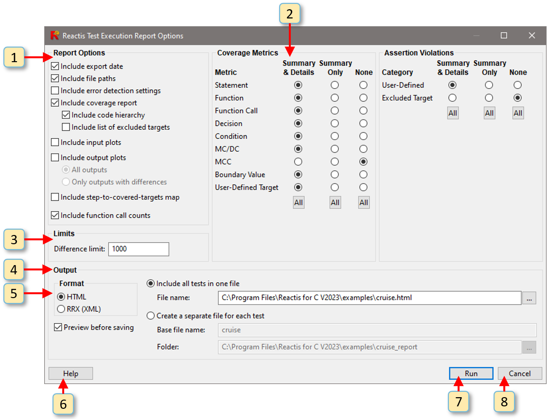
Fig. 8.2 The Reactis Test Execution Report Options dialog is used to select the items which appear in a test execution report.#
When Simulate > Fast Run with Report… is selected, the dialog shown in Figure 8.2 will appear. This dialog is used to select the items which will appear in the report. The following items are labeled in Figure 8.2:
The Report Options panel is used to select optional report items, such as the date, pathnames of input files, etc.
When Include coverage report is selected in the Report Options panel, the Coverage Metrics panel can be used to select which coverage metrics are included in the test execution report. There are three choices for each metric:
Summary & Details Targets of the metric will appear in both the coverage summary and coverage details sections of the report.
Summary Only Targets of the metric will appear in the coverage summary only.
None Targets of the metric will be omitted from the report entirely.
Note that due to dependencies between metrics, some combinations are not allowed. For example, Summary & Details cannot be selected for Condition targets unless Summary & Details is also selected for Decision targets.
The Difference limit prevents reports for test runs with many output differences from becoming excessively long. Once the limit is reached, output differences are still counted but no details are included in the report.
The Output panel determines where the report will be saved. When the output format is HTML, you can choose to save the results for each test in a separate file instead of generating a single file which contains the entire report.
The Output Format panel lets you choose between HTML and XML output formats. There is also an option to preview the results before saving the report.
Clicking on this button opens the help dialog.
When you are satisfied with the selected report options, clicking on this button will close the dialog and start the simulation run.
Clicking on this button will close the dialog without initiating a simulation run.
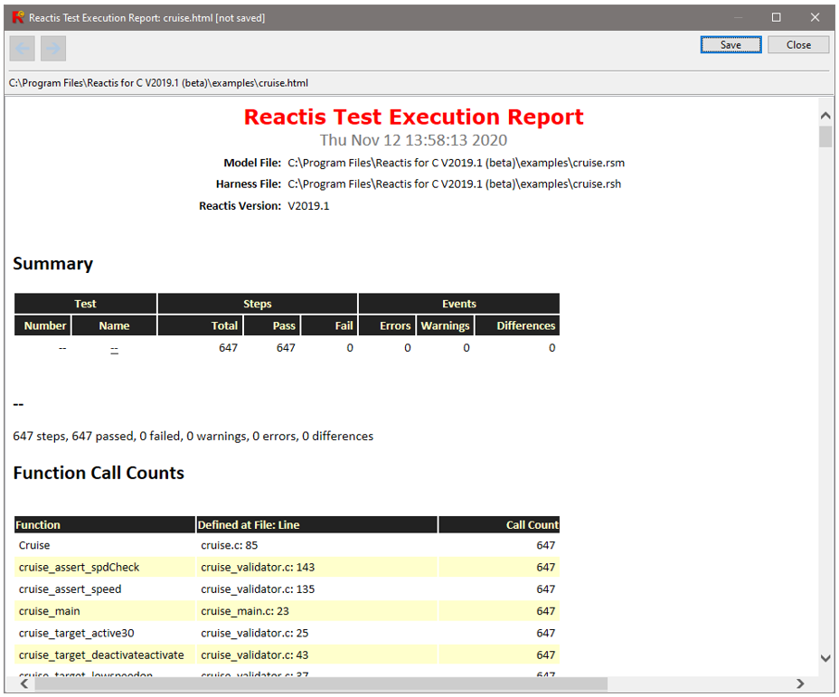
Fig. 8.3 A test execution report can be generated by loading a test suite in Simulator and selecting Simulate > Fast Run with Report…#
Once the simulation run begins, it does not stop until all tests have been executed. During each test, if a runtime error is encountered, the remaining steps of the test are skipped and Simulator continues execution with the following test. After the last test is executed, a window containing the test execution report will appear, as shown in Figure 8.3. An HTML version of the report can be saved by clicking the Save button in the report window.
An HTML test execution report will contain some or all of the following sections, depending on which options are selected:
A report header listing the data, input files, Reactis version, etc.
A test summary listing the tests/steps which were executed and the number of errors and differences detected for each test. Non-zero error and difference totals can be clicked-on to jump to a detailed description of the error or difference.
The tolerance used to test the value of each output and test point.
The error detection settings (e.g. integer overflow) used when generating the report.
A list of test details. For each test, includes the details for each error and difference that occurred, and plots of test data. The plots for a test are hidden by default, but they can be viewed by either clicking on the ± to the left of the signal name, or by clicking on Open all. See the Test Data Plots section for details.
The model hierarchy. The name of each member of the hierarchy can be clicked on to jump to the coverage details for that member.
Coverage details for each component of the model. The coverage details for a model component begin with a summary of the local and cumulative coverage, followed by details for each metric. The details for a metric show, for each target, whether or not the target was covered, and if the target was covered, the test step when coverage occurred. The contents of this section are identical to a coverage report. See Coverage Report Contents for information on coverage reports.
8.3.1. Test Data Plots#
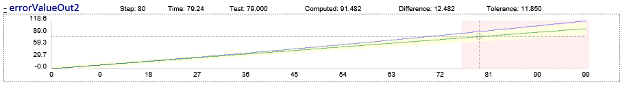
Fig. 8.4 An output plot from a test execution report.#
Figure 8.4 shows a typical plot from a test execution report. Test data (inputs, outputs, or test points) are plotted with the simulation time on the x-axis and the data value(s) on the y-axis. For outputs and test points, two values are shown: the test value (green), and the computed value (blue). The test value is the value stored in the test being executed for the output. The computed value is the value computed by the model for the output while executing the test. The acceptable tolerance between the two values is shaded yellow. Regions where the difference between the two signals is larger than the tolerance are shaded red.
Plots can be inspected when viewed from within a web browser or the preview dialog. The current focus of inspection is indicated by the intersection of two gray dashed lines. The focus can be moved either by the mouse, or the left and right arrow keys on the keyboard. Pressing S will move the focus to the start of the plot, and pressing E will move the focus to the end.
There are six values {^footnote4] displayed at the top of the plot for the current focus. These are (1) the step number, (2) the simulation time, (3) the test value (y value of green line), (4) the computed value (y value of blue line), (5) the difference between the test value and the computed value, and (6) the maximum difference between the test and computed values which is tolerated. These six values are updated whenever the focus is moved.
8.4. Specifying the Simulation Input Mode#
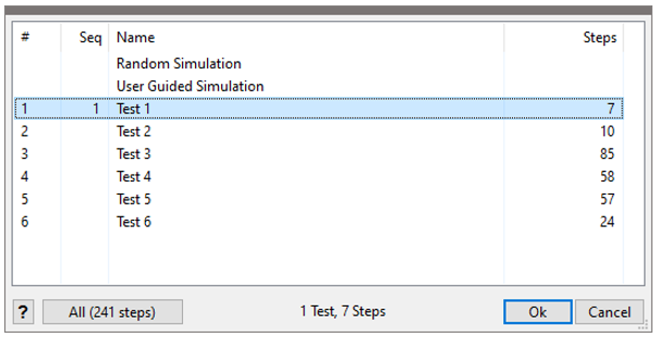
Fig. 8.5 The Source-of-Inputs Dialog enables you to specify how Simulator computes input values..#
Reactis Simulator performs simulations in a step-by-step manner: at each simulation step values are generated for each input, and resultant output values are reported. You control how Simulator computes input values using the Source-of-Inputs Dialog (window item 16 in Figure 8.1) shown in Figure 8.5. This dialog always includes the Random Simulation and User Guided Simulation entries; if a test suite has been loaded, then the dialog includes an entry for each test and the All button becomes enabled. The dialog is used to specify how input values are generated as follows.
- Random Simulation.
For each input, Reactis for C randomly selects a value from the set of allowed values for that variable, using type and probability information contained in the associated
.rshfile. See The Reactis Harness Editor for instructions on how to specify this information.- User Guided Simulation.
You determine the value for each input using the Next Input Value dialog, which appears when the User Guided Simulation entry is selected. See User Input Mode for more information on this mode.
- Individual Tests.
When a test suite is loaded, each test in the suite has a row in the dialog that contains a test number, a sequence number, a name and the number of steps in the test. Selecting a test and clicking on OK will cause inputs to be read from the test.
- Subset of Tests.
You may specify that a subset of tests should be run by holding down the control key and clicking on each test to be run with the left mouse button. The tests will be run in the order they are selected. As tests are selected the sequence number column is updated to indicate the execution order of the tests. When a new test is started, the code execution is reset to its starting configuration, although coverage information is not reset, thereby allowing users to view cumulative coverage information for the subset of tests.
- All Tests.
Clicking the All button in the lower left corner specifies that all tests in the suite should be executed one after another. The tests are executed sequentially. When a new test is started, the code execution is reset to its starting configuration, although coverage information is not reset, thereby allowing you to view cumulative coverage information for the entire test suite. For more information on this mode, see Test Input Mode.
You can change the sorting order of the tests in the table by clicking on the column headers. For example, to sort the tests by the number of steps, simply click on the header of the Steps column. Clicking again on that header will sort by number of steps in descending order.
You may also use the Source-of-Inputs Dialog to change the name of a test. To do so, select the test by clicking on it, then click on the name and, when the cursor appears, type in a new name.
8.4.1. User Input Mode#
When the User Guided Simulation mode is selected from the Source-of-Inputs dialog, you provide values for inputs at each execution step. This section describes how this is done.
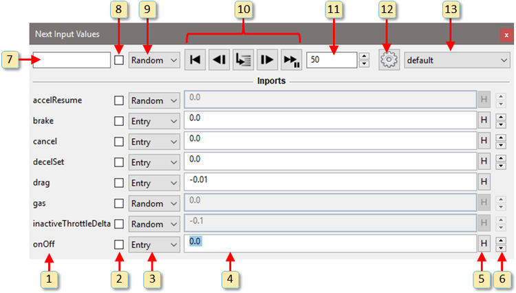
Fig. 8.6 The Next Input Values dialog lets you control the simulation by specifying the next value for inputs (item 4) and clicking the stepping buttons (item 10).#
To enter the user-guided mode of operation, select User Guided
Simulation from the Source-of-Inputs dialog (window item 16 in
Figure 8.1). Upon selecting user-guided
mode, a Next Input Values dialog appears, as shown in
Figure 8.6, that allows you to specify the input
values for the next simulation step. Initially, each top-level input
of the model has a row in the dialog. You can remove inputs from the
dialog or add outputs, test points, and configuration variables by
clicking the gear button  in the toolbar
of the Next Input Values dialog. Each row in the dialog contains 6
items (labeled 1-6 in Figure 8.6). The
toolbar for the dialog contains items 7-13. The elements of the dialog
work as follows:
in the toolbar
of the Next Input Values dialog. Each row in the dialog contains 6
items (labeled 1-6 in Figure 8.6). The
toolbar for the dialog contains items 7-13. The elements of the dialog
work as follows:
The name of an item (input, output, test point, or configuration variable).
This check box toggles whether the item is included in a scope displaying a subset of the signals from the Next Input Values dialog.
This pull-down menu has two entries that determine how the next value for the input is specified:
- Random
Randomly select the next value for the input from the type given for the input in the
.rshfile.- Entry
Specify the next value with the text-entry box in column four of the panel.
If the pull-down menu in column three is set to “Entry”, then the next input value is taken from this text-entry box. The entry can be a concrete value (e.g. integer or floating point constant) or a simple expression that is evaluated to compute the next value. These expressions can reference the previous values of inputs or the simulation time. For example, a ramp for input drag can be specified by pre(drag) + 0.0001. A sine wave can be generated by sin(t) * 0.001. For the full description of the expression notation, see Syntax of Next Input Value Expressions.
If the pull-down menu in column three is set to “Entry”, then clicking the history button (labeled H) displays recent values the input has assumed. Selecting a value from the list causes it to be placed in the text-entry box of column four.
The arrow buttons in this column enable scrolling through the possible values for the input. The arrows are available for inputs or configuration variables:
having a base type of integer, boolean or fixed point; or
having a base type of
doubleorsingleand either a resolution or subset of values constraint.
When you enter a search string in this box, Reactis displays only the rows for items whose names contains the given search string.
When you check this box, all signals in the Next Input Values dialog are plotted in a scope. When you uncheck this box, all signals are removed from the scope and no scope is displayed.
This pull-down menu sets the mode for all inputs at once to either “Random” or “Entry.”
These buttons control the simulation stepping exactly as they do in the top-level main Simulator window.
The entry in this box is a positive integer which specifies how many steps to take when clicking one of the stepping buttons that triggers multiple steps (e.g. fast simulation button).
Open a dialog to select the set of signals (inputs, outputs, test points, configuration variables) to be included in the Next Input Values dialog.
Save the current configuration of the Next Input Values dialog for future use or load a previously saved configuration.
When “run fast simulation” (window item 14 in Figure 8.1) is selected, the input value specifications in the Next Inputs Values dialog are used for each step in the simulation run.
8.4.1.1. Syntax of Next Input Value Expressions#
The value an input should assume in the next simulation step can be specified from its row by selecting Entry in column 3 and then entering an expression in the box in column 4. We now describe the language used to define an expression.
Assume foo is an input. Then the following examples demonstrate some possible expressions to specify the next value of foo.
Expression |
Value foo will have in next step |
|---|---|
4.0 |
4.0 |
pre(foo) |
The value foo had in the previous step |
pre(foo,2) |
The value foo had two steps back |
pre(foo) + 1 |
Add 1 to the value of foo in the previous step |
pre(u) |
Shorthand denoting the value of foo in the previous step |
t |
The current simulation time |
sin(t) |
The sine of current simulation time (i.e. generate a sine wave) |
The complete syntax of a next input value expression NIV is specified by the grammar shown in Table 8.1.
NIV |
: |
numericConstant | true | false C |
Constant value |
| |
inputName |
Name of an input (must be within pre) |
|
| |
u |
Shorthand for current input (must be within pre) |
|
| |
pre(NIV) |
Go one step back when retrieving values for inputs in NIV |
|
| |
pre(NIV,n) |
Go n steps back when retrieving values for inputs in NIV |
|
| |
t |
Simulation time |
|
| |
NIV relOp NIV |
Relational operator |
|
| |
! NIV |
Logical not |
|
| |
NIV && NIV |
Logical and |
|
| |
NIV || NIV |
Logical or |
|
| |
\(-\) NIV |
Negation |
|
| |
NIV arithOp NIV |
Arithmetic operation |
|
| |
function ( NIVL ) |
Function call |
|
| |
[ rowL ] |
Matrix |
|
| |
{ fieldL } |
Record |
|
| |
NIV . fieldName |
Access field of record |
|
| |
if NIV then NIV else NIV |
If then else |
|
| |
( NIV ) |
Parentheses |
|
relOp |
: |
< | <= | == | != | >= | > |
|
arithOp |
: |
\(+\) | \(-\) | \(*\) | \(/\) |
|
field |
: |
fieldName = NIV |
|
function |
: |
abs | fabs |
Absolute value |
| |
sin | cos | tan | asin | acos | atan | atan2 | sinh | cosh |
Trigonometric functions |
|
| |
floor | ceil |
Rounding functions |
|
| |
hypot(a,b) |
Calculate length of hypotenuse c, if a and b are lengths of non-hypotenuse sides of right triangle. |
|
| |
ln | log | log10 | pow | exp |
Log and exponent functions |
|
| |
rem | sgn | sqrt |
||
NIVL |
: |
list of NIV delimited by , |
|
rowL |
: |
list of NIVL delimited by ; |
|
fieldL |
: |
list of field delimited by , |
8.4.1.2. Reading Data from Existing Test Suites in Expressions#
Within the expression for specifying the next input value for a port the testval_step and testval_time functions can be used to read values from an existing test suite.
- testval_step(suitefilename, portname, testnum, stepnum)
Reads a value from a test suite, specified by the step number within the test suite.
- testsuitefilename
The file name of the test suite from which data should be read. If a relative path is used then it is relative to the directory in which the current model resides. Must be enclosed in double-quotes.
- portname
The name of the port from which data should be read. This can be an input port, test point or output port, as they appear in the Reactis Test Suite browser. You can use the function “port()” here to use the same name as the port whose input you are specifying. The name must be enclosed in quotes.
- testnum
The number of the test in the test suite from which data should be read. This number is 1-based, i.e. first step is 1.
- stepnum
The step number within the test. Use the “step()” function to refer to the current simulation step. You can use arithmetic expressions to adjust the step number, for example to add an offset.
Example: testval_step(”cruise.rst”, “onOff”, 3, step()+5) will read data from the 3rd test of test suite “cruise.rst”, port “onOff”, offset by 5 steps, i.e. the first step read from the test suite will be step 6.
- testval_time(suitefilename, portname, testnum, time, interpolate)
Reads a value from a test suite, specified by the simulation time in the test suite.
- testsuitefilename
The file name of the test suite from which data should be read. If a relative path is used then it is relative to the directory in which the current model resides. Must be enclosed in double-quotes.
- portname
The name of the port from which data should be read. This can be an input port, test point or output port, as they appear in the Reactis Test Suite browser. You can use the function “port()” here to use the same name as the port whose input you are specifying. The name must be enclosed in quotes.
- testnum
The number of the test in the test suite from which data should be read. This number is 1-based, i.e. first step is 1.
- time
The simulation time within the test. Use “t” to refer to the current simulation model time. You can use arithmetic expressions to adjust the time value, for example to add an offset or scaling.
- interpolate
If the time value specified falls between the time for two steps in the test suite then this parameter defines how the value is computed. If the interpolate parameter is 0 then the value from the test suite corresponding to the step before the time value is used. If interpolate is 1 then the value is interpolated (linear) between the steps before and after the simulation time.
Example: testval_time(”cruise.rst*”, port(), 4, t/10, 1) will read data from the 4th test of test suite “cruise.rst” matching the current port name. Time will be slowed down by factor 10 and values will be interpolated between steps.
8.4.1.3. Select Signals Dialog#
The Select Signals dialog lets you choose which signals to include in
the Next Input Values dialog during user-guided simulation. Initially
all harness inputs are included, but you can remove inputs or add outputs,
test-points, and configuration variables by clicking the
button in the Next Input Values dialog
and then using the Select Signals dialog to specify the desired subset
of signals. Note that in the case of outputs and test points the signal
values are only observed, not controlled.
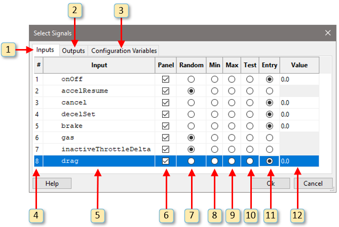
Fig. 8.7 The Select Signals dialog lets you choose the subset of signals to include in the Next Input Values dialog during user-guided simulation.#
The labeled items in Figure 8.7 work as follows. Note that since outputs and test points are only observed and not controlled, those tabs include only a subset of the columns described below.
This tab lets you select harness inputs.
This tab lets you select harness outputs.
This tab lets you select configuration variables.
Port number.
Signal name.
Toggles whether or not the item is included in the Next Input Values dialog.
Generate a random next input value.
Generate the smallest allowed next input value.
Generate the largest allowed next input value.
Reads a value from an existing test suite (see the Reading Data From Existing Test Suites section).
Use an expression in item 12 to specify the next input value.
An expression used to generate the next input value.
Note that if item 7 is checked for an input, then the settings specified by items 8-10 will determine the initial configuration of the Next Input Values when it is first opened. The settings can subsequently be modified while stepping. If window item 7 is not checked for an input, then the settings specified by items 8-10 will be the only ones used during stepping.
8.4.1.4. Reading Data from Existing Test Suites#
In user-guided simulation mode you can set up any number of inputs to read data from one or more existing test suites:
To set all inputs to receive data from the same test suite, either select the “Test” entry in the “all ports” drop-down box in the Next Input Values window (item 9 in Figure 8.6) or click on the header of the “Test” column in the Select Signals dialog (item 11 in Figure 8.7).
To set a single input to receive data from a test suite, either select the “Test” entry in the drop-down box for the desired input in the Next Input Values window (item 3 in Figure 8.6) or click the radio button in the “Test” column for the desired input in the Select Signals dialog (item 11 in Figure 8.7).
To set a range of inputs to receive data from the same test suite, open the Select Signals dialog (Figure 8.7) and click in the “Test” column of the first input to be set to a test. Make your selections in the test selection dialog (see below) and click Ok. Then hold down the shift key and click the last input to be set to a test, which will again bring up the test selection dialog, pre-configured with your previous selection. Click the Ok button again.
Doing any of the above will bring up the dialog shown in Figure 8.8, the labeled items work as follows.
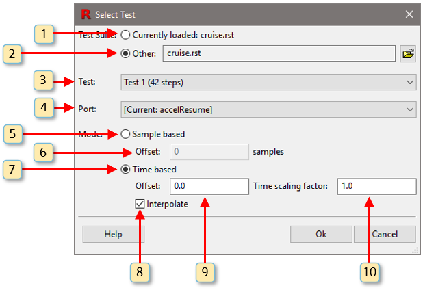
Fig. 8.8 Selecting data to be read from a test suite.#
Test data will be read from the test suite currently loaded in Simulator. Note that the test suite must be saved before it can be selected here.
Test data will be read from the test suite selected here.
Selects the test from which data will be read
Data item (input port, output port, configuration variable or test point) in the test suite that the data will be read from. If set to “[Current]” then data will be read from the port in the test suite whose that matches the current port name. This choice is disabled when selecting test data for multiple inputs.
If this mode is selected then data will be read from the test suite on a step-by-step basis, disregarding simulation time. This mode is more efficient and avoids possible rounding errors if the sample rate of the model and the data in the test suite are identical. If test data is read for steps past the end of the test data, the last step value will be repeated.
This allows to set an offset to the step number in the test suite. For example, if set to 5 then the first step read from the test suite will be step number 6. If this is a negative value then the data read before step 1 will be the same as the data for step 1.
If this mode is selected then data will be read from the test suite based on the current simulation time. This is useful if either the sample rate of the test data does not match the model’s sample rate or to perform time scaling (see below).
If this is checked and the time from which data is to be read from the test falls between two time steps in the test suite then linear interpolation will be used to calculate the test data value. If this is not checked then the data from the previous step in the test suite will be used. This also influences the behavior if test data is read for time less than zero or past the end of the test. If checked then the two first or last steps in the test data are used to extrapolate the test data value for the given time. Otherwise the test data for the first or last step is used.
Provide a time offset when reading data from the test suite. This value will be added to the current simulation time to determine the time for which data is read from the test suite.
Provide a time scaling when reading data from the test suite. The current simulation time will be multiplied by this value (before adding the offset) to determine the time for which data is read from the test suite. This allows to speed up or slow down time. For example, if set to 0.5 then data from the test suite will be read at half the speed at which the model simulation time progresses.
Note that this dialog is meant to provide a more user-friendly way to specify the parameters to the testval_step() and testval_time() functions described above in the Reading Data from Existing Test Suites in Expressions section. Using the functions directly will provide more flexibility in how to read test data. If you set up a port to read data from a test using this dialog and subsequently switch the test data selector (item 3 in Figure 8.6) to “Entry” then you will see the function expression that was constructed to reflect your dialog choices.
8.4.2. Test Input Mode#
Simulation inputs may also be drawn from tests in a Reactis test
suite. Such tests may be generated automatically by Reactis Tester,
constructed manually in Reactis Simulator, or imported using a comma
separated value file format. By convention files storing Reactis test
suites have names suffixed by .rst.
A Reactis test suite may be loaded into Simulator by clicking the
 in the toolbar to the right of
Source-of-Inputs Dialog (window item 18 in Figure 8.1) or by selecting the Test Suite > Open menu item.
in the toolbar to the right of
Source-of-Inputs Dialog (window item 18 in Figure 8.1) or by selecting the Test Suite > Open menu item.
When a test suite is loaded, the name of the test suite appears in the Reactis for C title bar and the tests of the suite are listed in the Source-of-Inputs Dialog.
When executing in test input mode while Test Suite > Compare Outputs is selected, after each simulation step, Simulator compares the values computed by the code against the values stored in the test suite for those items. Any difference is flagged if it exceeds the tolerance specified for that output. See the Tolerance Editor Dialog section for more information on specifying tolerances for outputs.
8.5. Tracking Data-Item Values#
Reactis Simulator includes several facilities for interactively displaying the values that data items assume during simulation. The watched-variable list, or “watch list” for short, displays the current values of data items designated by the user as “watched variables.” You may also attach scopes to global or static local variables in order to display their values at the end of a simulation step plotted on a graph with time on the horizontal axis. Scopes let you easily see how a variable changes during a simulation run. Distribution scopes enable you to view the set of values a data item has assumed during simulation (but not the time at which they occur).
Difference scopes may be opened for harness outputs when reading inputs from a test in order to plot the values computed by the program under test against the values stored in the test for the output.
You may add data items to the watch list, or attach scopes to them, by right-clicking on a data item in the Reactis main panel and selecting an entry from the resulting menu as described in the Labeled Window Items section.
You may save the current configuration of the data tracking facilities
(the variables in the watch list and currently open scopes along with
their locations) for use in a future Simulator session. You do so, by
selecting View > Save Profile As… and using the resulting file
selection dialog to specify a file in which to save a Reactis profile
(.rsp file ). The profile may be loaded at a future time by selecting
View > Load Profile….
8.5.1. Viewing Item Details#
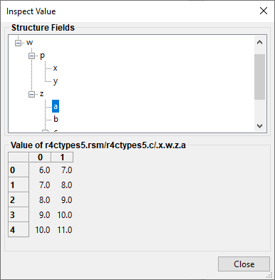
Fig. 8.9 Inspecting the value of a structure.#
When you right-click on an item in the main panel and select View Item Details, a dialog similar to Figure 8.9 will appear displaying the same information that can be viewed by hovering on the item. This is useful for items with a very large amount of information (e.g., a structure with many members). You can also copy some or all of the data in the View Item Details dialog to the clipboard if desired.
8.5.2. Selecting Variable Components#
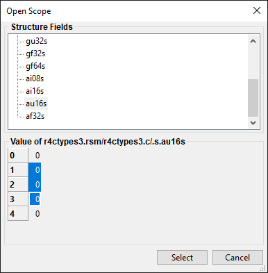
Fig. 8.10 Opening a scope on a component of a structure.#
When any of the standard value-inspection operations (Inspect
value…, Add Watched Variables…, Open Scopes… , Open
Distribution Scopes…) are applied to a structure or array, an
intermediate menu appears which allows you to select one or more
components of interest. An example of this is shown in
Figure 8.10, where the second, third, and
fourth elements of s.au16s are about to be selected.
8.5.3. The Watched-Variable List#
The watch list is displayed in a panel at the bottom of the Simulator screen as shown in Figure 3.12. By default this panel is hidden, although adding a variable to the watch list causes the panel to become visible. Visibility of the panel may also be toggled using the View menu as described in the menus section. The panel displays a list of data items and their values. The values are updated when Simulator pauses.
The contents of the watch list may be edited using a pop-up menu that is activated from inside the watch-list panel. Individual data items in the panel may be selected by left-clicking on them. Once an item is selected, right-clicking invokes a pop-up menu that enables the selected item(s) to be deleted, have a scope opened, or have a distribution scope opened. If no item is selected, then these choices are grayed out. The right-click pop-up menu also includes an entry Add Variables which displays a list of all data items in the program under test which may be added to the watch list.
The View menu contains operations for displaying / hiding the watch list, adding data items to the watch list, clearing the watch list.
8.5.4. Scopes#
Scopes appear in separate windows, an example of which may be found in Figure 8.11. The toolbar of each scope window contains nine or more items.
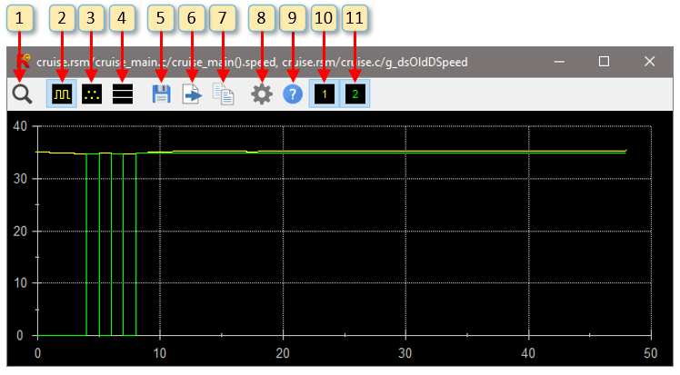
Fig. 8.11 A scope window plotting desired speed (green) and actual speed (yellow).#
- Labeled Window Items
Reset the zoom level of the scope to fit the whole plot (see more on zooming below).
Plot signal as solid lines.
Plot signal as points.
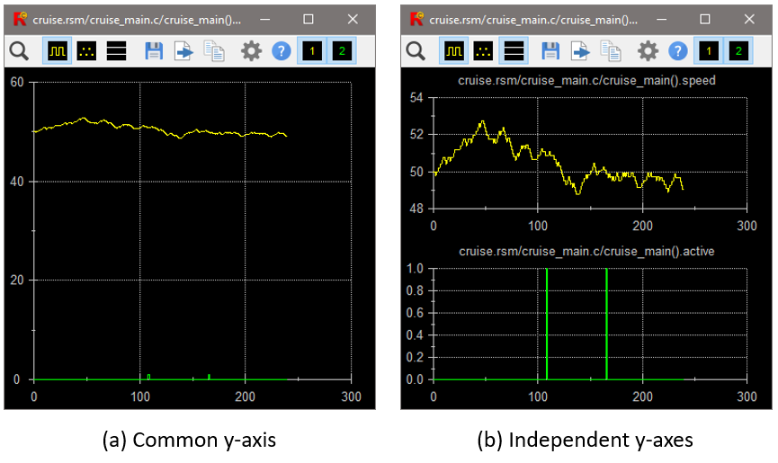
Fig. 8.12 Scopes showing multiple signals can be plotted using a single y-axis (a) or separate y-axes (b).#
If a scope displays multiple signals, this button toggles whether or not all signals share the same y-axis (Figure 8.12 (a)), or each is plotted on its own y-axis (Figure 8.12 (b)).
Save the current scope configuration as a signal group. A signal group is a set of signals along with the settings for displaying the signals in a scope. After saving a signal group, you can reopen a scope for the group in future Reactis sessions. You can add additional signals to a signal group by right-clicking on a signal in the main Reactis panel (when Simulator is enabled), selecting Add to Scope, and selecting the signal group to be extended. To reorder the signals in a group or remove a signal, open a scope for the signal group then click the Settings button (item 8).
Export scope data as either text (csv) or graphics (png, gif, bmp, tif or jpg).
Copy a screen shot of the scope to the clipboard.
Configure the scope settings, including reordering the signals or deleting a signal.
Display help for scopes.
Toggle display of signal 1.
Toggle display of signal 2.
To zoom in to a region of interest of the signal shown in the scope, left-click the top-left corner of the region, hold the button and drag to the lower right corner of the region. The scope will zoom in to the selected region. To zoom out, either click the zoom-to-fit button in the toolbar or right-click in the scope window. Right-clicking will return to the zoom level that was active before the last zoom.
When zoomed in, it is possible to move the displayed region within the scope window. To move the region, hold down the CTRL key and click-and-drag with the left mouse button.
If more than one data item is plotted on a scope, then a toggle button will appear in the toolbar for each data item (window items 10 and 11 in Figure 8.11). Turning one of these buttons off will hide the corresponding data item in the scope. Hovering over the button will display the data item to which the button corresponds.
8.5.5. Distribution Scopes#
Distribution scopes also appear in separate windows, an example of which may be found in Figure 8.13. The values a data item assumes are displayed as data points distributed across the X-axis. Zooming in distribution scopes works the same as in regular scopes.
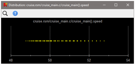
Fig. 8.13 Distribution scopes plot the values a data item has assumed during simulation.#
8.5.6. Difference Scopes#
When executing tests from a test suite, a difference scope may be opened by right-clicking on a test harness output and selecting Open Difference Scope. The resulting scope plots the expected value (from the test) against the actual value (computed by the program under test), as shown in Figure 8.14. If the difference between the two values exceeds the tolerance specified for the output (see Tolerance Methods for more information on how tolerances work), then a red background in the difference scope and a red bar on the X-axis highlight the difference.
After zooming into an area of difference, white and yellow and green background regions around the plotted values highlight the tolerance, as shown in Figure 8.15. The green region represents the overlap between the tolerance of the test and model values. A difference is flagged whenever the test or model value lie outside of the green region.
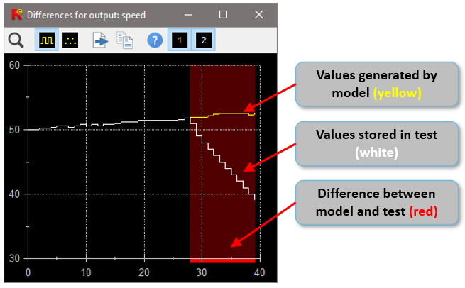
Fig. 8.14 A difference scope may be opened by right-clicking on a test harness output and selecting Open Difference Scope. The scope plots the values stored in a test for an output and the values computed by the program for the output. Differences are flagged in red.#
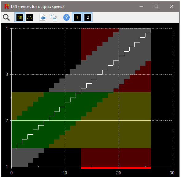
Fig. 8.15 The white and yellow colored backgrounds around the value lines highlight the tolerance intervals of the test and model values. The overlap between the yellow and white regions is colored green. If either the test or program value lie outside the green region, a difference is flagged.#
8.6. Tracking Code Coverage#
The Reactis Coverage Metrics chapter describes the coverage metrics that Reactis for C employs for measuring how many of a given class of syntactic constructs or coverage targets that appear in the code have been executed at least once. Simulator includes extensive support for viewing this coverage information about the parts of the code that have been exercised by the current simulation run. If a test suite is being executed the coverage data is cumulative. That is all targets covered by the portion of the current test executed so far, plus those targets exercised in previous tests are listed as covered.
8.6.1. The Coverage Summary Dialog#
The Coverage Summary Dialog shown in Figure 8.16 may be invoked at any time Simulator is enabled by selecting Coverage > Show Summary. The dialog reports summary statistics for each coverage criterion tracked by Reactis. Each row in the dialog corresponds to one of the criterion and includes five columns described below from left to right.
The name of the coverage criterion reported in the row.
The number of targets in the criterion that have been exercised at least once.
The number of targets in the criterion that are unreachable. A conservative analysis is performed to check for unreachable targets. Any target listed as unreachable is provably unreachable; however, some unreachable targets might not be flagged as unreachable.
The number of reachable targets in the criterion that have not been exercised.
The percentage of reachable targets in the criterion that have been exercised at least once.
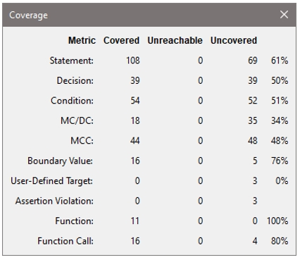
Fig. 8.16 The coverage summary dialog.#
8.6.2. Coverage Information in the Main Panel#
Selecting Coverage > Show Details toggles the highlighting of uncovered targets in the main panel. Targets that have been covered are drawn in black, while red implies an uncovered target. Please refer to the Reactis Coverage Metrics chapter for a detailed description of how the different coverage metrics are highlighted in the main panel.
Hovering over an exercised target will cause a pop-up to be displayed
that gives the test and step in which the target was first
executed. This type of test and step coverage information is displayed
with a message of the form test/step. A “.” appearing in the test
position ./step denotes the current simulation run which has not yet
been added to a test suite.
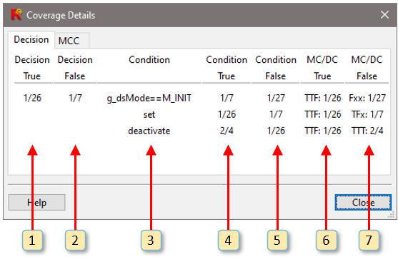
Fig. 8.17 Viewing coverage details for a decision.#
For items included in the decision, condition, MC/DC, and MCC metrics, detailed coverage information may be obtained by right-clicking on the item and selecting View Coverage Details. A dialog similar to the one shown in Figure 8.17 will appear with coverage information. This dialog has two tabs, one titled Decision which contains Decision, Condition, and MC/DC details, and a second named MCC which contains MCC details.
Item 1 in Figure 8.17 shows the coverage details dialog with the Decision tab selected. The table within this tab describes the coverage status of all decision, condition, and MC/DC targets for the following decision:
g_dsMode==M_INIT && (set && !deactivate)
This decision contains three conditions: g_dsMode==M_INIT, set, and
!deactivate. Conditions are the atomic Boolean expressions that are
used in decisions (for more details on decisions and conditions, see
the Decision Coverage section and the
Condition Coverage section).
Each decision details table contains seven columns, numbered 1-7 in Figure 8.17. These are interpreted as follows:
The test/step during which the decision first evaluated to true.
The test/step during which the decision first evaluated to false.
The conditions from which the decision is composed.
The test/step during which the condition first evaluated to true.
The test/step during which the condition first evaluated to false.
The condition values and test/step during which an MC/DC target was covered and the decision evaluated to true.
The condition values and test/step during which an MC/DC target was covered and the decision evaluated to false.
Note that although all targets were covered in Figure 8.17, this will not necessarily be the every time you view the details of a decision, in which case a test/step value of -/- will indicate that a target has not yet been covered.
MC/DC requires that each condition independently affect the outcome of
the decision in which it resides. (See the MCDC Coverage
section for additional details.) When a condition has met the MC/DC criterion
in a set of tests, columns 6 and 7 of the table explain how. Each
element of these two columns has the form bbb:test/step, where each
b reports the outcome of evaluating one of the conditions in the
decision during the test and step specified. Each b is either T to
indicate the condition evaluated to true, F to indicate the
condition evaluated to false, or x to mean the condition was not
evaluated due to short circuiting.
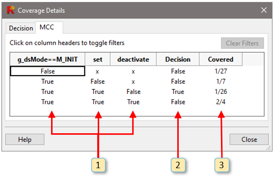
Fig. 8.18 Viewing MCC details for a decision.#
In addition to the MC/DC, Reactis can also measure Modified Condition Coverage, or MCC.MCC targets every possible combination of conditions within a decision, so that a decision containing N conditions can result in as many as \(2^N\) MCC targets, although the actual number may be less if short-circuited evaluation is used.
Figure 8.18 shows the coverage details dialog with the MCC tab selected. Each row of this table corresponds to a single MCC target. The table columns are interpreted as follows:
Each of these columns corresponds to a condition. Every condition within the decision is always represented by a single column in the table. For each target, all conditions have one of three possible values:
- True.
The condition is true.
- False.
The condition is false.
- x.
The condition is not evaluated due to short-circuiting.
The next-to-last column contains the decision outcomes for each MCC target.
The last column gives the test/step in which the MCC target was covered.
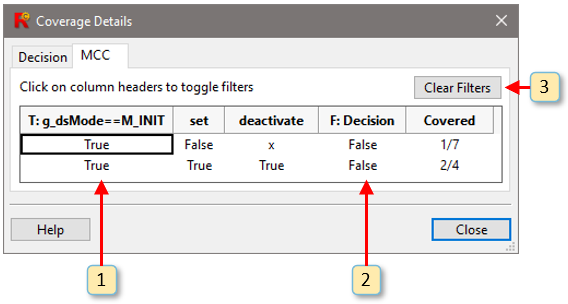
Fig. 8.19 Filtering MCC coverage information.#
MCC coverage details can be filtered by clicking on the column
headers, as shown in Figure 8.19. A
filtered column header is indicated by a prefix of T:, F:, or x:,
which correspond to the column values True, False, and x,
respectively. In Figure 8.19, items
1 and 2 refer to columns with active filters:
Only MCC targets for which the condition
g_dsMode==M_INITevaluated to true are being shown, as indicated by theT:prefix in the header for this column.Only MCC targets for which the decision evaluated to false are being shown, as indicated by the
F:prefix in the header for this column.
Clicking on a column header advances the filter setting for that column to the next feasible value, eventually cycling back to unfiltered. All columns can also be reset to the unfiltered state at any time by clicking on the Clear Filter button (item 3 in Figure 8.19). Note that the individual filters for each column are combined exclusively (i.e., using the Boolean and operator), so that only targets which satisfy all active filters are shown.
8.6.3. The Coverage Report Browser#
The Coverage-Report Browser enables you to view detailed coverage information and export the reports in HTML format. It is invoked by selecting Coverage > Show Report and is described in detail in The Reactis Coverage-Report Browser chapter.
8.7. Exporting and Importing Test Suites#
8.7.1. Exporting Test Suites#
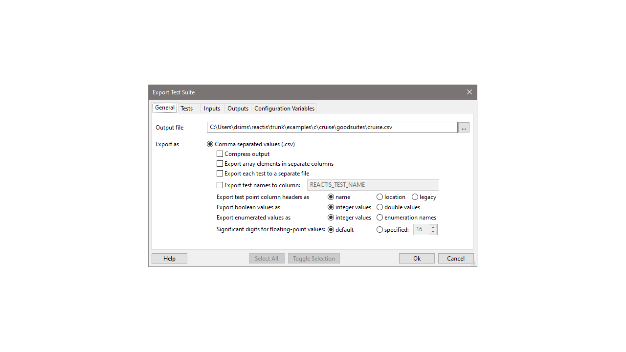
Fig. 8.20 The Reactis test-suite export window.#
The export feature of Reactis for C allows you to save .rst files in
different formats so that they may be processed easily by other
tools. The feature is launched by selecting Test Suite > Export…
when a test suite is loaded in Simulator. You specify the format and
name of the exported file in the General tab of the Export Dialog
(Figure 8.20). For some export formats, other
tabs appear in the dialog to enable you to fine-tune exactly what is
included in the exported file. In the case of .csv files, you may
specify a subset of tests from the test suite to be exported as well
as which data items (inputs, outputs, configuration variables) should
be included in each test step. The following formats are currently
supported:
- .csv files:
Suites may be saved as comma separated value (CSV) files. The different tabs of the export dialog enable you to specify which data from a test suite should be exported. Namely, you can indicate which tests should be exported and for each test step which inputs, outputs, and configuration variables should have values recorded.
If the Compress output check box is selected, then test steps will be omitted if no item that would be recorded in the step is different from the corresponding value in the previously recorded step. This is especially useful when exporting only input data for a test in which inputs are held constant for a number of steps.
The first line of an exported file will contain a comma separated list of the names of the harness inputs, outputs, and configuration variables that were selected for export. A column recording the simulation time has the label t. Any names containing non-alphanumeric characters will be surrounded by double quotes (”) and newlines in names will be translated to
\n.After the first line, subsequent lines contain either:
A comma-separated list of values that includes one value for each item appearing in the first row. The order of the values in a row corresponds to the order the items appeared in the first line. Each such line contains the values for one simulation step. For array valued items, the elements of the array appear within double quotes (”) as a comma-separated list.
An empty line signaling the end of a test.
- .txt files:
Suites may be saved in a more verbose plain ASCII format to facilitate inspection of the test data.
8.7.2. Creating Test Suite Templates#
A Test Suite Template is a CSV file which contains columns for each element of a test suite, but does not contain any data. This can be useful when you wish to convert test data from an external source into a CSV format which can be easily imported into Reactis. To create a template, start Simulator and then select Test Suite > Create Template…. This will open a dialog similar to the one shown in Figure 8.21.
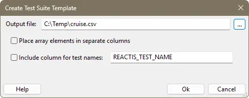
Fig. 8.21 The Create Test Suite Template dialog.#
When using the Export Test Suite dialog, the first step is to select the name of the file which will be created. There are then two options which you can select:
Place array elements in separate columns. When selected, this will produce a separate column for each array element. The column names will include the array index values. If this option is not selected, then a single column will be created for an array value, with the expectation that cell in the column will contain the value for the entire array.
Include column for test names. When selected, this will add an extra column using the name in the text box to the right of the checkbox. As shown in Figure 8.21, the default name is REACTIS_TEST_NAME. This column is expected to contain a string value for the first row of each test which gives the name assigned to the test. The name can be left empty.
8.7.3. Importing Test Suites#
Reactis can also import tests and add them to the current test
suite. Test suites may be imported if they are stored in the Reactis’
native .rst file format or in the comma separated value (CSV) format
(described above) that Reactis exports. The import feature is launched
by selecting Test Suite > Import… when Simulator is enabled.
To execute a test suite in Simulator, the test suite must match the
currently selected harness. A test suite matches a harness if it
contains data for the same set of inputs, outputs, and configuration
variables as the harness. If an externally visible data item (input,
output, or configuration variable) is added to or removed from the
harness, then previously constructed test suites will no longer match
the new version of the harness. The import facility gives you a way to
transform the old test suite so that it matches the new version of the
harness. Such remapping is also available when importing .csv files.
The Import Dialog, shown in Figure 8.22, is used to
specify how test data should be remapped during import. The dialog
contains a tab for each type of data item stored in a test suite
(inputs, outputs, configuration variables). In the case of .csv files,
the import dialog also contains a tab Not Imported that lists items
present in the CSV file that are not scheduled to be imported. When an
.rst file includes an item not scheduled to be imported, it is placed
at the bottom of the appropriate tab. For example, if a test suite
contains an input variable X and is being imported with respect to a
harness that has no input variable X, then X will appear at the bottom
of the Input variables tab and be highlighted in yellow.
Each data item tab (e.g. Inputs) includes a column (e.g. Harness Input Name) listing the code elements in that category. The Suite column lists items from the file being imported that map to the corresponding harness item. In most cases a data item X in the test suite being imported will map to an item with the same name in the harness. If the harness contains an item not found in the test suite being imported, then the corresponding Suite column entry will be listed as Random Value and be highlighted in yellow (as shown in Figure 8.22 for input brake). If this setting is not changed, then upon import a random value will be generated for the input at each test step. The value to be mapped to any harness item may be changed by double clicking on the corresponding entry in the Suite column (alternatively selecting the item and clicking the button Select Suite Item) and then using the resulting dialog to either select an item from the test suite being imported or set it to Random Value.
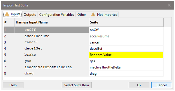
Fig. 8.22 The Import Test Suite dialog.#
8.8. Updating Test Suites#
Test Suite > Update… creates a new test suite that retains the inputs from the current test suite, but updates the outputs with values computed by the execution of your code on the existing inputs. This provides a means to reuse previously constructed test suites when your code changes in a way that causes its externally visible behavior to change.